How to reuse the model you already trained (Forecast, version 13)?
This is the last note in the forecasting series. Version 12 trained two hundred models and saved
the winner's weights in a file called best_model_12.pt. Version 13 trains nothing at
all: it rebuilds the same network, loads those saved weights, and reports the same four scores in
a few seconds.
What is actually saved
The last line of version 12's model section is
torch.save(best_trial["model"].state_dict(), "best_model_12.pt"). A
state_dict is a dictionary of numbers: the weights and biases of each layer, named
after the layer they belong to. It holds no program and no settings, and the file is a little over
half a megabyte.
So the file cannot rebuild itself. Version 13 has to supply the shape — how many layers, how
wide, and how long the window. It builds an empty network of that shape, and then
load_state_dict copies the saved numbers into it. If the shape does not match,
PyTorch stops with an error rather than producing a wrong forecast.
Where the config comes from
Near the top of version 13 the settings are not typed in. They are read from the table that version 12 wrote:
RESULTS_FILE = "search_results_12.xlsx"
MODEL_FILE   = "best_model_12.pt"
BATCH_SIZE   = 32

results  = pd.read_excel(RESULTS_FILE)
best_row = results.sort_values("r2", ascending=False).iloc[0]

BEST_CFG = {
    "window_size": int(best_row["window_size"]),
    "hidden_size": int(best_row["hidden_size"]),
    "num_layers":  int(best_row["num_layers"]),
}
read_excel loads the 200-row table. Sorting it by r2, highest first,
and taking .iloc[0] picks the winning row, and the three settings that decide the
shape are copied out by column name. int() turns them into plain integers, because
layer sizes must be plain integers.
Only three of the six settings are needed. Epochs, learning rate and optimizer belong to a training run, and this program does not train. Because the table is read rather than typed, if version 12 is rerun and a different combination wins, this program follows the new winner by itself.
How the program works
1. Rebuild the data with the same window size
window_size = BEST_CFG["window_size"]
windows     = series_tensor.unfold(0, window_size, 1)
features    = windows[:, :-1]
targets     = windows[:, -1:]
full_dataset = TensorDataset(features, targets)

total   = len(full_dataset)
val_end = int(total * 0.85)
test_loader = DataLoader(Subset(full_dataset, range(val_end, total)),
                         batch_size=BATCH_SIZE, shuffle=False)
The windows and the test split are built exactly as explained in How wide should the search be (version 12), with one difference: only the test loader is built, because nothing is being trained.
2. Rebuild the architecture and load the weights
def build_model(input_size, hidden_size, num_layers):
    layers, in_dim = [], input_size
    for _ in range(num_layers):
        layers += [nn.Linear(in_dim, hidden_size), nn.ReLU()]
        in_dim = hidden_size
    layers.append(nn.Linear(in_dim, 1))
    return nn.Sequential(*layers)

model = build_model(window_size - 1, BEST_CFG["hidden_size"], BEST_CFG["num_layers"])
model.load_state_dict(torch.load(MODEL_FILE, map_location=device))
model.to(device)
model.eval()
The network is built exactly as in
How wide should the search be (version 12), so its shape matches the
saved file. The line that matters is
model.load_state_dict(torch.load(MODEL_FILE, map_location=device)):
torch.load reads the file and load_state_dict copies every saved number
into the matching layer. map_location places those numbers on whichever device is
available, and model.to(device) moves the network to the same place.
model.eval() switches it to test mode.
3. Run the test days through the saved model
preds, actuals = [], []
with torch.no_grad():
    for xb, yb in test_loader:
        preds.extend(model(xb.to(device)).cpu().numpy())
        actuals.extend(yb.numpy())
torch.no_grad() tells PyTorch that nothing is being learned here. The program is only
making predictions, not improving the model, so this setting saves time and memory. The
predictions and the true values stay in the same order, because the loader does not shuffle them.
model.eval() puts the network into testing mode. Some kinds of layers behave
differently while training and while testing, and this setting selects the testing behaviour.
This network has only simple layers, so it makes no difference here, but it keeps the program
correct if another kind of layer is added later.
Because the model is already trained, you can also use it on different data. Put the new sales values in a CSV file in the same format, keep the same window size, and run the program again. It loads the saved weights and produces predictions for those new days instead of the 217 test days.
4. Compute the four measures
mae  = torch.mean(torch.abs(p - a)).item()
mse  = torch.mean((p - a) ** 2).item()
rmse = torch.sqrt(torch.tensor(mse)).item()
r2   = (1 - torch.sum((a - p) ** 2) / torch.sum((a - torch.mean(a)) ** 2)).item()
MAE averages the size of the misses, MSE squares them first, and RMSE takes the square root so the number is back in sales dollars. R² compares the model with always predicting the average of the test days, as explained in How to measure the model on data it has never seen (version 8).
What you should see
The complete output of a real run, unedited:
Loaded: best_model_12.pt
Config: {'window_size': 20, 'hidden_size': 256, 'num_layers': 3}

Test Set Metrics:
  MAE:  4.1235
  MSE:  26.7236
  RMSE: 5.1695
  R²:   0.4790
Saved: best_model_predictions.png
The four numbers match what version 12 printed for its winner exactly, to the fourth decimal place. Nothing was trained, nothing was shuffled, and no random seed took part in the scoring. The same weights on the same 217 days give the same answer, which is what a saved model is for.
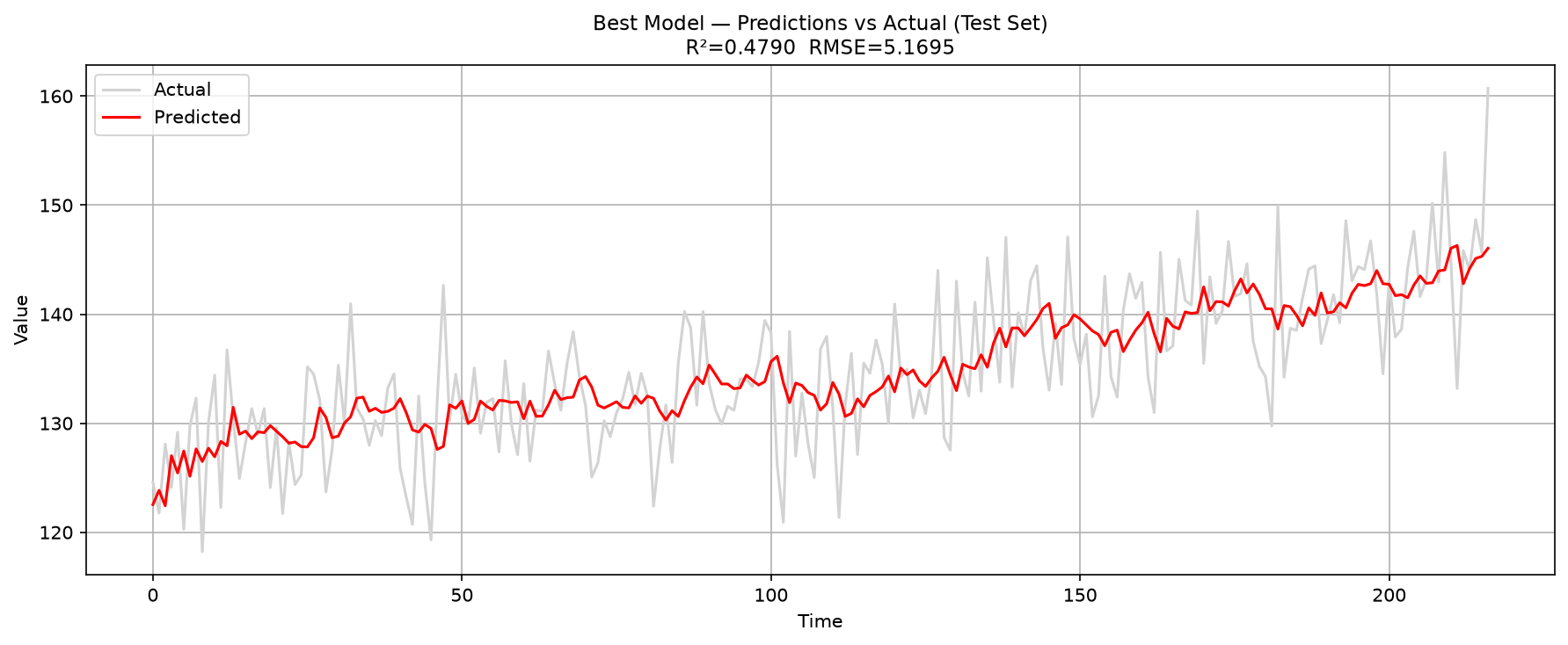
best_model_12.pt and running no training. The chart is titled with R² 0.4790 and RMSE 5.1695.The series in one view
Thirteen programs, one question: what will the next day's sales be, given the recent past? Versions 1 to 3 looked at the data and cut it into windows. Versions 4 to 6 turned those windows into features and targets and split them in date order, so that the model is always graded on days that come after the days it learned from. Version 7 trained a network. Version 8 graded it honestly on days it had never seen. Versions 9 to 12 searched settings — how long to train, how big a step to take, which optimiser, how wide, how deep, how far back — ending with two hundred trials. Version 13 kept the result and showed how to pick it up again.
What the model can do is modest: it follows the level and the slow upward drift of the series, turning 19 past values into one number in a fraction of a second. It cannot follow the daily swings; an R² of about 0.48 means roughly half of the variation in the test days is still unexplained. The network sees only the recent sales values, so it does not know the day of the week, the month or a holiday.
A better next step is not a bigger search but better inputs or a different kind of model, such as
one that can remember longer patterns. One obstacle comes first: the time column in
time_series.csv is a step number from 1 to 1,460, not a date, so day-of-week and month
cannot be worked out until real dates are attached to the rows.
The whole program
The pieces above, put back together. This is the complete file:
import os
os.environ["KMP_DUPLICATE_LIB_OK"] = "TRUE"

import torch
import torch.nn as nn
import pandas as pd
import numpy as np
import matplotlib.pyplot as plt
from torch.utils.data import TensorDataset, DataLoader, Subset

# ── Best config, read from search_results_12.xlsx (Rank 1) ───────────────────
RESULTS_FILE = "search_results_12.xlsx"
MODEL_FILE   = "best_model_12.pt"
BATCH_SIZE   = 32

results  = pd.read_excel(RESULTS_FILE)
best_row = results.sort_values("r2", ascending=False).iloc[0]

BEST_CFG = {
    "window_size": int(best_row["window_size"]),
    "hidden_size": int(best_row["hidden_size"]),
    "num_layers":  int(best_row["num_layers"]),
}

# ── Load data ─────────────────────────────────────────────────────────────────
df = pd.read_csv("time_series.csv")
series = df["series"].values
series_tensor = torch.tensor(series, dtype=torch.float32)

window_size = BEST_CFG["window_size"]
windows     = series_tensor.unfold(0, window_size, 1)
features    = windows[:, :-1]
targets     = windows[:, -1:]
full_dataset = TensorDataset(features, targets)

total   = len(full_dataset)
val_end = int(total * 0.85)
test_loader = DataLoader(Subset(full_dataset, range(val_end, total)),
                         batch_size=BATCH_SIZE, shuffle=False)

device = torch.device("cuda" if torch.cuda.is_available() else "cpu")

# ── Rebuild model architecture & load weights ─────────────────────────────────
def build_model(input_size, hidden_size, num_layers):
    layers, in_dim = [], input_size
    for _ in range(num_layers):
        layers += [nn.Linear(in_dim, hidden_size), nn.ReLU()]
        in_dim = hidden_size
    layers.append(nn.Linear(in_dim, 1))
    return nn.Sequential(*layers)

model = build_model(window_size - 1, BEST_CFG["hidden_size"], BEST_CFG["num_layers"])
model.load_state_dict(torch.load(MODEL_FILE, map_location=device))
model.to(device)
model.eval()
print(f"Loaded: {MODEL_FILE}")
print(f"Config: {BEST_CFG}\n")

# ── Evaluate ──────────────────────────────────────────────────────────────────
preds, actuals = [], []
with torch.no_grad():
    for xb, yb in test_loader:
        preds.extend(model(xb.to(device)).cpu().numpy())
        actuals.extend(yb.numpy())

p = torch.tensor(np.array(preds))
a = torch.tensor(np.array(actuals))

mae  = torch.mean(torch.abs(p - a)).item()
mse  = torch.mean((p - a) ** 2).item()
rmse = torch.sqrt(torch.tensor(mse)).item()
r2   = (1 - torch.sum((a - p) ** 2) / torch.sum((a - torch.mean(a)) ** 2)).item()

print(f"Test Set Metrics:")
print(f"  MAE:  {mae:.4f}")
print(f"  MSE:  {mse:.4f}")
print(f"  RMSE: {rmse:.4f}")
print(f"  R²:   {r2:.4f}")

# ── Plots ─────────────────────────────────────────────────────────────────────
# 1. Predictions vs actual
plt.figure(figsize=(12, 5))
plt.plot(actuals, label="Actual",    color="lightgrey", linewidth=1.5)
plt.plot(preds,   label="Predicted", color="red",       linewidth=1.5)
plt.title(f"Best Model — Predictions vs Actual (Test Set)\nR²={r2:.4f}  RMSE={rmse:.4f}", fontsize=11)
plt.xlabel("Time"); plt.ylabel("Value")
plt.legend(); plt.grid(True)
plt.tight_layout()
plt.savefig("best_model_predictions.png", dpi=150)
plt.show()
print("Saved: best_model_predictions.png")
Running it on your own computer
Download the zip file and unzip it
to a folder. The zip holds the programs in this series, the time_series.csv
data file and pyproject.toml. This note uses time_13.py.
Version 13 has one requirement that no earlier note had: it needs
best_model_12.pt, and that file exists only after time_12.py has
been run once in the same folder. Version 12 runs two hundred trials and needs a good while
to finish.
Version 13 takes seconds, because it does none of that work.
Open the folder in Visual Studio Code, then type these three lines in the terminal:
uv python pin 3.12.10
uv sync
uv run time_13.py
The first line records which Python version this folder uses, and the second installs every
package that pyproject.toml lists. The third line loads the saved weights,
prints the four scores and draws one chart, saving it as
best_model_predictions.png; close the window when you have looked at it.
Those three lines are needed only once. The next time you want to run the program again,
type just uv run time_13.py.
If you have not set up uv yet, start with How to install Visual Studio Code? and then the uv note for Windows or Mac.