How to measure the model on data it has never seen (Forecast, version 8)?
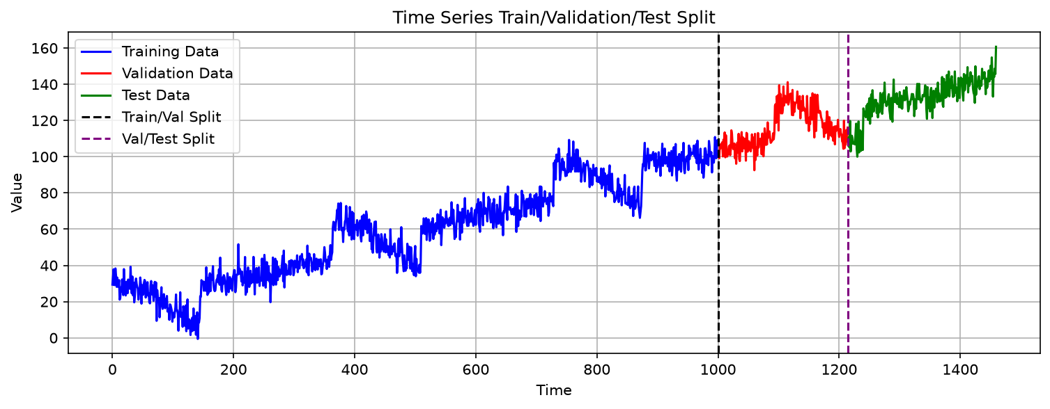
This is version 8 of the forecasting series. Version 7 judged the model on validation days, but those days were also used, epoch after epoch, to decide when training looked good. That makes them no longer fully fair. Version 8 therefore cuts the data into three parts instead of two — training, validation and test — keeps the test part sealed until the very end, and reports four numbers on it.
Why three parts, not two
The validation days are used while training is still going on. After every epoch, the program measures their loss, so you can see whether the model is improving or beginning to memorise. These results also guide your decisions: whether to train for more epochs and, in later versions, which settings to choose. Because the validation results influence those decisions, they stop being a completely independent check. It is like using the same practice exam repeatedly: a good score may reflect familiarity with those particular questions rather than how well you would do on new ones.
The test part deals with that problem by being kept out of the room. It is sealed before training starts, opened once after training has finished, and used for nothing except the final report. No decision along the way was made with it in view, so whatever it says is an honest answer to the question how good is this model on days it has never seen?
Where the three cuts fall
train_size = int(total_windows * 0.7)
val_size = int(total_windows * 0.15)
test_size = total_windows - train_size - val_size
1,431 examples give train_size of 1,001 (0.7 of 1,431 is 1,001.7, and
int() drops the decimal) and val_size of 214. The test part takes
whatever is left rather than its own percentage, so the three parts always add back to 1,431:
1,001 + 214 + 216.
The three lists of positions are again three unbroken stretches of time, earliest first, so the model trains on the oldest days, is watched on the middle ones, and is graded on the newest.
The four measures
All four compare the model's guesses with the real days in the test part, and each answers a slightly different question.
- MAE — mean absolute error: the average size of a miss, in dollars. Easy to explain, and it is about 5.03 here.
- MSE — mean squared error: the same misses squared. Big misses count far more than small ones, which is useful when a large error is much worse than a small one, but the units are dollars squared, which nobody can picture.
- RMSE — root mean squared error: the square root of MSE, which puts the number back into dollars. About 6.23 here, and always a little larger than MAE because squaring lets one bad day weigh heavily.
- R² — the fraction of the day-to-day variation the model explains. 1 is perfect; 0 means the model does no better than replying with the average every day.
R² of 0.24 here is the number worth staring at. The model is clearly better than guessing the average, but it accounts for only about a quarter of the movement in the test days. This is an honest, modest result, and versions 9 and 10 try to improve it.
How the program works
1. Build three loaders
train_indices = list(range(train_size))
val_indices = list(range(train_size, train_size + val_size))
test_indices = list(range(train_size + val_size, total_windows))

train_dataset = Subset(full_dataset, train_indices)
val_dataset = Subset(full_dataset, val_indices)
test_dataset = Subset(full_dataset, test_indices)

batch_size = 32
train_loader = DataLoader(train_dataset, batch_size=batch_size, shuffle=True)
val_loader = DataLoader(val_dataset, batch_size=batch_size, shuffle=False)
test_loader = DataLoader(test_dataset, batch_size=batch_size, shuffle=False)
Version 6's two-way split becomes three, with the same shape: three lists of positions, three
Subsets, three loaders. Training shuffles; the other two do not, so their
measurements stay comparable from run to run.
2. Train exactly as before
The network, the loss, the optimizer and the 100-epoch loop are unchanged from version 7. Only the split above and the measurement below are new. That is worth noticing: once the training loop exists, adding a fair test does not require touching it.
3. Measure once, after training
model.eval()
test_predictions = []
test_targets = []
with torch.no_grad():
    for batch_features, batch_targets in test_loader:
        batch_features = batch_features.to(device)
        outputs = model(batch_features)
        test_predictions.extend(outputs.cpu().numpy())
        test_targets.extend(batch_targets.numpy())
The two lists collect the guesses and the real answers over the whole test part. .extend
adds every batch's contents to the list, so that at the end the two lists hold 216 numbers
each, in order.
4. Turn the lists into the four numbers
mae = torch.mean(torch.abs(test_predictions_tensor - test_targets_tensor))
mse = torch.mean((test_predictions_tensor - test_targets_tensor) ** 2)
rmse = torch.sqrt(mse)
ss_res = torch.sum((test_targets_tensor - test_predictions_tensor) ** 2)
ss_tot = torch.sum((test_targets_tensor - torch.mean(test_targets_tensor)) ** 2)
r2 = 1 - ss_res / ss_tot
Each line is the definition written out. MAE averages the absolute differences; MSE averages the squared differences; RMSE takes the square root of MSE.
R² compares the model with a simple alternative: if we did not have a useful model, we
could use the average sales value of the test days as the prediction for every day.
ss_res is the total squared error from the model, and ss_tot is the
total squared error from this average-based prediction. Dividing one by the other shows how
much error remains compared with the simple average, and subtracting from 1 shows how much
error the model removes.
If the model performs no better than the average-based prediction, the two totals are equal,
the ratio is 1, and R² is 0. If the model is perfect, ss_res is 0 and
R² is 1.
What you should see
Epoch [10/100], Train Loss: 45.0302, Val Loss: 53.8099
Epoch [20/100], Train Loss: 45.5068, Val Loss: 51.7960
Epoch [30/100], Train Loss: 43.4795, Val Loss: 54.2412
Epoch [40/100], Train Loss: 42.1594, Val Loss: 50.4357
Epoch [50/100], Train Loss: 40.0044, Val Loss: 47.8687
Epoch [60/100], Train Loss: 38.7391, Val Loss: 45.2560
Epoch [70/100], Train Loss: 37.1991, Val Loss: 44.5767
Epoch [80/100], Train Loss: 36.1731, Val Loss: 41.6744
Epoch [90/100], Train Loss: 35.9192, Val Loss: 42.3977
Epoch [100/100], Train Loss: 33.9332, Val Loss: 45.6109

Test Set Metrics:
  MAE:  5.0289
  MSE:  38.7685
  RMSE: 6.2264
  R²:   0.2404
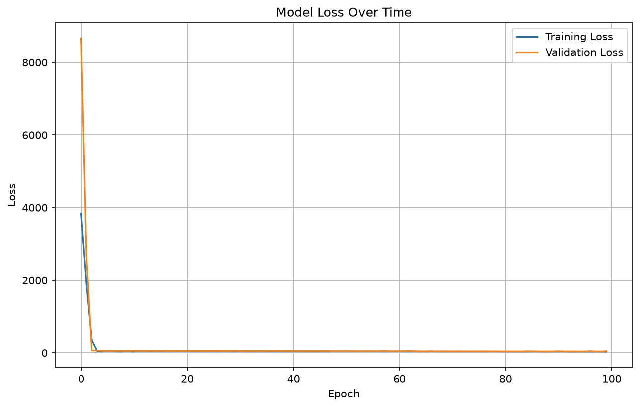
As in version 7, your numbers will differ from these because the weights start at random. The pattern to look for is that the training loss keeps falling while the validation loss flattens and wobbles, and that RMSE sits somewhat above MAE.
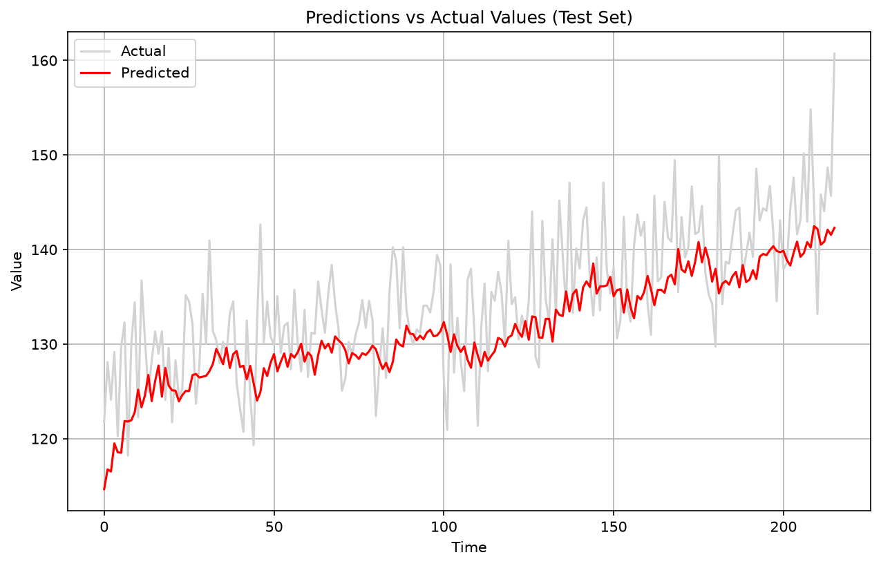
In the second chart the red line follows the general rise but flattens out the peaks. A model that cannot reach the peaks is exactly what an R² of 0.24 looks like on a picture.
The whole program
The pieces above, put back together. This is the complete file:
import torch
from torch.utils.data import TensorDataset, DataLoader, Subset
import pandas as pd
import matplotlib.pyplot as plt

def create_sliding_windows_with_target(data, window_size, shift=1):
    windows = data.unfold(0, window_size, shift)
    features = windows[:, :-1]
    targets = windows[:, -1:]
    return features, targets

df = pd.read_csv('time_series.csv')
series = df['series'].values
series_tensor = torch.tensor(series, dtype=torch.float32)
window_size = 30
features, targets = create_sliding_windows_with_target(series_tensor, window_size=window_size, shift=1)
full_dataset = TensorDataset(features, targets)

total_windows = len(full_dataset)
train_size = int(total_windows * 0.7)
val_size = int(total_windows * 0.15)
test_size = total_windows - train_size - val_size

train_indices = list(range(train_size))
val_indices = list(range(train_size, train_size + val_size))
test_indices = list(range(train_size + val_size, total_windows))

train_dataset = Subset(full_dataset, train_indices)
val_dataset = Subset(full_dataset, val_indices)
test_dataset = Subset(full_dataset, test_indices)

batch_size = 32
train_loader = DataLoader(train_dataset, batch_size=batch_size, shuffle=True)
val_loader = DataLoader(val_dataset, batch_size=batch_size, shuffle=False)
test_loader = DataLoader(test_dataset, batch_size=batch_size, shuffle=False)

# Visualize train/val/test split
val_start = train_size
test_start = train_size + val_size
plt.figure(figsize=(12, 4))
plt.plot(range(val_start), series[:val_start], 'b-', label='Training Data')
plt.plot(range(val_start, test_start), series[val_start:test_start], 'r-', label='Validation Data')
plt.plot(range(test_start, len(series)), series[test_start:], 'g-', label='Test Data')
plt.axvline(x=val_start, color='k', linestyle='--', label='Train/Val Split')
plt.axvline(x=test_start, color='purple', linestyle='--', label='Val/Test Split')
plt.title('Time Series Train/Validation/Test Split')
plt.xlabel('Time')
plt.ylabel('Value')
plt.legend()
plt.grid(True)
plt.show()

import torch.nn as nn
import torch.optim as optim

class TimeSeriesModel(nn.Module):
    def __init__(self, window_size):
        super(TimeSeriesModel, self).__init__()
        self.network = nn.Sequential(
            nn.Linear(window_size - 1, 10),
            nn.ReLU(),
            nn.Linear(10, 10),
            nn.ReLU(),
            nn.Linear(10, 1)
        )

    def forward(self, x):
        return self.network(x)

model = TimeSeriesModel(window_size)
criterion = nn.MSELoss()
optimizer = optim.Adam(model.parameters())

num_epochs = 100
device = torch.device('cuda' if torch.cuda.is_available() else 'cpu')
model.to(device)

train_losses = []
val_losses = []

for epoch in range(num_epochs):
    model.train()
    train_loss = 0
    for batch_features, batch_targets in train_loader:
        batch_features = batch_features.to(device)
        batch_targets = batch_targets.to(device)
        outputs = model(batch_features)
        loss = criterion(outputs, batch_targets)
        optimizer.zero_grad()
        loss.backward()
        optimizer.step()
        train_loss += loss.item()

    model.eval()
    val_loss = 0
    with torch.no_grad():
        for batch_features, batch_targets in val_loader:
            batch_features = batch_features.to(device)
            batch_targets = batch_targets.to(device)
            outputs = model(batch_features)
            val_loss += criterion(outputs, batch_targets).item()

    train_loss /= len(train_loader)
    val_loss /= len(val_loader)
    train_losses.append(train_loss)
    val_losses.append(val_loss)

    if (epoch + 1) % 10 == 0:
        print(f'Epoch [{epoch+1}/{num_epochs}], '
              f'Train Loss: {train_loss:.4f}, '
              f'Val Loss: {val_loss:.4f}')

# Plot training progress
plt.figure(figsize=(10, 6))
plt.plot(train_losses, label='Training Loss')
plt.plot(val_losses, label='Validation Loss')
plt.title('Model Loss Over Time')
plt.xlabel('Epoch')
plt.ylabel('Loss')
plt.legend()
plt.grid(True)
plt.show()

# Evaluate on test set
model.eval()
test_predictions = []
test_targets = []
with torch.no_grad():
    for batch_features, batch_targets in test_loader:
        batch_features = batch_features.to(device)
        outputs = model(batch_features)
        test_predictions.extend(outputs.cpu().numpy())
        test_targets.extend(batch_targets.numpy())

# Plot predictions vs actual for test set
plt.figure(figsize=(10, 6))
plt.plot(test_targets, label='Actual', color='lightgrey')
plt.plot(test_predictions, label='Predicted', color='red')
plt.title('Predictions vs Actual Values (Test Set)')
plt.xlabel('Time')
plt.ylabel('Value')
plt.legend()
plt.grid(True)
plt.show()

# Metrics on test set
test_predictions_tensor = torch.tensor(test_predictions)
test_targets_tensor = torch.tensor(test_targets)

mae = torch.mean(torch.abs(test_predictions_tensor - test_targets_tensor))
mse = torch.mean((test_predictions_tensor - test_targets_tensor) ** 2)
rmse = torch.sqrt(mse)
ss_res = torch.sum((test_targets_tensor - test_predictions_tensor) ** 2)
ss_tot = torch.sum((test_targets_tensor - torch.mean(test_targets_tensor)) ** 2)
r2 = 1 - ss_res / ss_tot

print(f"\nTest Set Metrics:")
print(f"  MAE:  {mae:.4f}")
print(f"  MSE:  {mse:.4f}")
print(f"  RMSE: {rmse:.4f}")
print(f"  R²:   {r2:.4f}")
Running it on your own computer
Download the zip file and unzip it
to a folder. The zip holds the programs in this series so far, the
time_series.csv data file, and pyproject.toml. This note uses
time_08.py. Open the folder in Visual Studio Code, then type these three lines
in the terminal:
uv python pin 3.12.10
uv sync
uv run time_08.py
The first line records which Python version this folder uses, and the second installs every
package that pyproject.toml lists. The third line prints the epoch lines and the
four test measures, and opens three chart windows in turn; close each one to continue.
Those three lines are needed only once. The next time you want to run the program again,
type just uv run time_08.py.
If you have not set up uv yet, start with How to install Visual Studio Code? and then the uv note for Windows or Mac.
What comes next
An R² of 0.24 leaves plenty of room. Version 9 stops guessing at the settings and tries several learning rates by hand, with early stopping, and keeps whichever one scores best.