How wide should the search be (Forecast, version 12)?
Version 11 searched six dials with twenty trials. Version 12 keeps the same six dials but widens every one of them, then runs 200 trials instead of 20. That change is small on paper and large in practice, because this is the point in the series where the cost of searching becomes real. Ten times the trials means roughly ten times the waiting, and the answer it buys is not ten times better.
A wider space and a bigger budget
The search space in the file is the honest source for all of this. It reads:
SEARCH_SPACE = {
    "epochs":       [100, 200, 300, 500],
    "learning_rate":[0.0001, 0.001, 0.005, 0.01, 0.05, 0.1],
    "optimizer":    ["Adam", "SGD", "RMSprop"],
    "hidden_size":  [10, 32, 64, 128, 256],
    "num_layers":   [1, 2, 3, 4],
    "window_size":  [10, 20, 30, 50],
}
Count the values in each list and multiply: 4 × 6 × 3 × 5 × 4 × 4 =
5,760 possible combinations. Version 11 offered 972. The budget line underneath is
N_TRIALS = 200, so the program draws 200 of those 5,760 at random and trains each
one. That is a little under 3.5 per cent of the space.
What "diverged" means
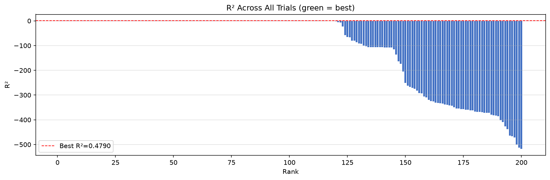
R² is measured against a simple alternative: predicting the average sales value for every day. That comparison is explained in How to measure the model on data it has never seen (version 8). A score of 1.0 is a perfect forecast. A score of 0.0 is exactly as good as that average-based prediction. A negative score is worse. So a large negative number is not a near miss. It means the model's guesses were further from the truth than a flat average line would have been. In practice, the weights changed too much during training and the errors did not become smaller. The program does not treat this as an error. It records the score and moves on to the next trial.
What you should see
The real run printed 200 rows. The table below is trimmed to twelve of them: the twelve printed
here include the winner, several respectable trials and four of the collapses. The
Trial numbers are positions in the original run order, so they are not consecutive.
Running 200 random trials...

Trial   Win  Epochs      LR      Opt  Hidden  Layers        R2        RMSE
------------------------------------------------------------------------------
    1    30     500    0.01  RMSprop      64       2    0.4421      5.3064
    2    10     100    0.01  RMSprop      64       1    0.4529      5.3201
    4    20     200    0.01      SGD      10       4  -341.2371    132.4929
    9    50     500     0.1     Adam      32       2   -91.9151     68.3195
   14    10     100   0.001     Adam      32       2    0.4612      5.2795
   27    10     300   0.005     Adam     256       4    0.4616      5.2777
   32    20     100  0.0001     Adam     128       2    0.4646      5.2406
   70    20     300  0.0001  RMSprop     256       3    0.4790      5.1695
   89    20     200   0.005      SGD      10       2  -465.9302    154.7587
   95    20     500     0.1      SGD      64       2  -470.9389    155.5865
  168    10     200    0.05     Adam      64       4    0.4660      5.2561
  185    30     100   0.001  RMSprop     256       3    0.4733      5.1559

Best model saved → best_model_12.pt
Best config : {'epochs': 300, 'learning_rate': 0.0001, 'optimizer': 'RMSprop', 'hidden_size': 256, 'num_layers': 3, 'window_size': 20}

Test Set Metrics:
  MAE:  4.1235
  MSE:  26.7236
  RMSE: 5.1695
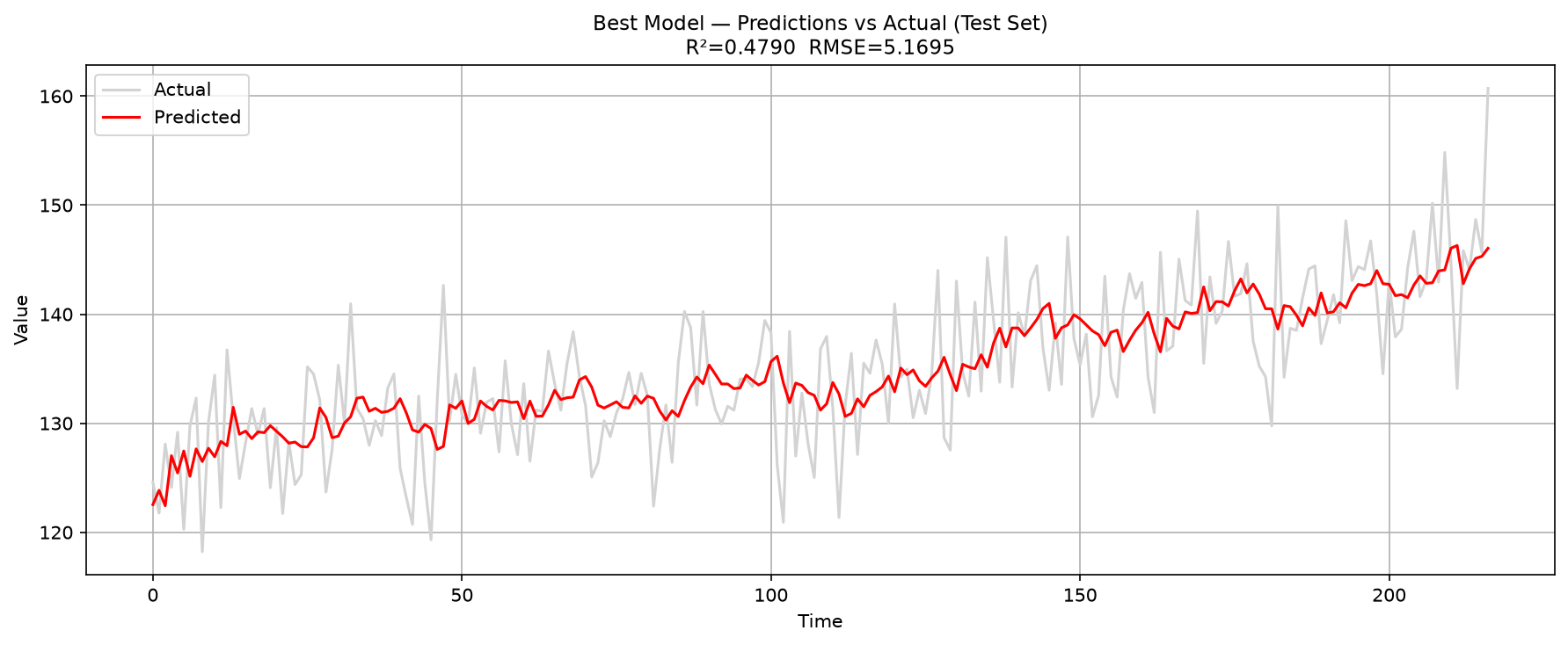
  R²:   0.4790

Results table saved → search_results_12.xlsx
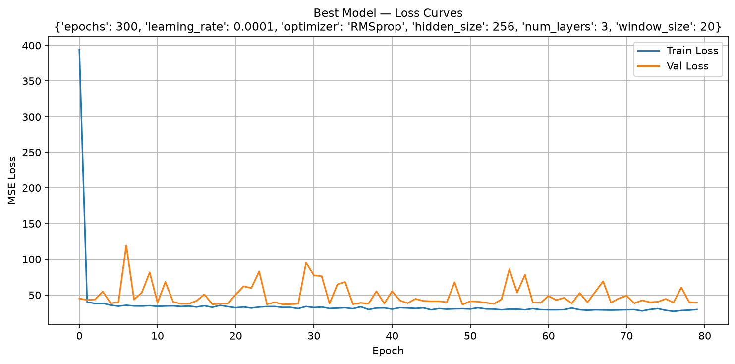
Trial 70 is the winner: 300 epochs, learning rate 0.0001, RMSprop, 256 hidden units, 3 layers and a window of 20. Early stopping ended its training after 80 of the 300 allowed epochs, so the extra epochs in the setting were never used.
Two hundred trials bought 0.0217 of R². Version 11's best was 0.4573 and this one is 0.4790, so ten times the computing moved the score by 0.0217.
Best-of-20 and best-of-200 are not the same measurement. A larger draw has more chances of catching a lucky configuration.
The winner takes very small steps. The smallest learning rate on offer, 0.0001, won with 0.4790.
The window answer also moved: version 11 pointed at a window of 10, while this larger search points at 20.
The whole program
The file below is the complete time_12.py, unedited:
import os
os.environ["KMP_DUPLICATE_LIB_OK"] = "TRUE"

import torch
import torch.nn as nn
import torch.optim as optim
from torch.utils.data import TensorDataset, DataLoader, Subset
import pandas as pd
import numpy as np
import matplotlib.pyplot as plt
import random
import itertools

# ── Reproducibility ──────────────────────────────────────────────────────────
SEED = 42
random.seed(SEED)
np.random.seed(SEED)
torch.manual_seed(SEED)

# ── Search space ─────────────────────────────────────────────────────────────
SEARCH_SPACE = {
    "epochs":       [100, 200, 300, 500],
    "learning_rate":[0.0001, 0.001, 0.005, 0.01, 0.05, 0.1],
    "optimizer":    ["Adam", "SGD", "RMSprop"],
    "hidden_size":  [10, 32, 64, 128, 256],
    "num_layers":   [1, 2, 3, 4],
    "window_size":  [10, 20, 30, 50],
}
N_TRIALS            = 200
EARLY_STOP_PATIENCE = 30
BATCH_SIZE          = 32

# ── Data ─────────────────────────────────────────────────────────────────────
df = pd.read_csv("time_series.csv")
series = df["series"].values
series_tensor = torch.tensor(series, dtype=torch.float32)

def make_loaders(window_size):
    windows      = series_tensor.unfold(0, window_size, 1)
    features     = windows[:, :-1]
    targets      = windows[:, -1:]
    full_dataset = TensorDataset(features, targets)
    total        = len(full_dataset)
    tr_end       = int(total * 0.70)
    val_end      = int(total * 0.85)
    train_loader = DataLoader(Subset(full_dataset, range(tr_end)),           batch_size=BATCH_SIZE, shuffle=True)
    val_loader   = DataLoader(Subset(full_dataset, range(tr_end, val_end)),  batch_size=BATCH_SIZE, shuffle=False)
    test_loader  = DataLoader(Subset(full_dataset, range(val_end, total)),   batch_size=BATCH_SIZE, shuffle=False)
    return train_loader, val_loader, test_loader

device = torch.device("cuda" if torch.cuda.is_available() else "cpu")

# ── Model factory ─────────────────────────────────────────────────────────────
def build_model(input_size, hidden_size, num_layers):
    layers = []
    in_dim = input_size
    for _ in range(num_layers):
        layers += [nn.Linear(in_dim, hidden_size), nn.ReLU()]
        in_dim = hidden_size
    layers.append(nn.Linear(in_dim, 1))
    return nn.Sequential(*layers).to(device)

def get_optimizer(name, params, lr):
    return {"Adam": optim.Adam, "SGD": optim.SGD, "RMSprop": optim.RMSprop}[name](params, lr=lr)

# ── Train one trial ───────────────────────────────────────────────────────────
def train_trial(cfg):
    train_loader, val_loader, test_loader = make_loaders(cfg["window_size"])
    model     = build_model(cfg["window_size"] - 1, cfg["hidden_size"], cfg["num_layers"])
    criterion = nn.MSELoss()
    optimizer = get_optimizer(cfg["optimizer"], model.parameters(), cfg["learning_rate"])

    best_val_loss = float("inf")
    best_state    = {k: v.clone() for k, v in model.state_dict().items()}
    patience_ctr  = 0
    train_losses, val_losses = [], []

    for epoch in range(cfg["epochs"]):
        # train
        model.train()
        t_loss = 0
        for xb, yb in train_loader:
            xb, yb = xb.to(device), yb.to(device)
            optimizer.zero_grad()
            loss = criterion(model(xb), yb)
            loss.backward()
            optimizer.step()
            t_loss += loss.item()
        t_loss /= len(train_loader)

        # validate
        model.eval()
        v_loss = 0
        with torch.no_grad():
            for xb, yb in val_loader:
                v_loss += criterion(model(xb.to(device)), yb.to(device)).item()
        v_loss /= len(val_loader)

        train_losses.append(t_loss)
        val_losses.append(v_loss)

        # early stopping
        if v_loss < best_val_loss:
            best_val_loss = v_loss
            best_state    = {k: v.clone() for k, v in model.state_dict().items()}
            patience_ctr  = 0
        else:
            patience_ctr += 1
            if patience_ctr >= EARLY_STOP_PATIENCE:
                break

    model.load_state_dict(best_state)
    return model, train_losses, val_losses, test_loader

# ── Evaluate on test set ──────────────────────────────────────────────────────
def evaluate(model, test_loader):
    model.eval()
    preds, actuals = [], []
    with torch.no_grad():
        for xb, yb in test_loader:
            preds.extend(model(xb.to(device)).cpu().numpy())
            actuals.extend(yb.numpy())
    p = torch.tensor(np.array(preds))
    a = torch.tensor(np.array(actuals))
    mae  = torch.mean(torch.abs(p - a)).item()
    mse  = torch.mean((p - a) ** 2).item()
    rmse = torch.sqrt(torch.tensor(mse)).item()
    ss_res = torch.sum((a - p) ** 2)
    ss_tot = torch.sum((a - torch.mean(a)) ** 2)
    r2 = (1 - ss_res / ss_tot).item()
    return r2, mae, mse, rmse, preds, actuals

# ── Random search ─────────────────────────────────────────────────────────────
keys   = list(SEARCH_SPACE.keys())
combos = list(itertools.product(*SEARCH_SPACE.values()))
sampled = random.sample(combos, min(N_TRIALS, len(combos)))

results = []
best_r2    = -float("inf")
best_trial = None

print(f"Running {N_TRIALS} random trials...\n")
print(f"{'Trial':>5}  {'Win':>4}  {'Epochs':>6}  {'LR':>6}  {'Opt':>7}  {'Hidden':>6}  {'Layers':>6}  {'R2':>8}  {'RMSE':>10}")
print("-" * 78)

for i, combo in enumerate(sampled):
    cfg = dict(zip(keys, combo))
    model, t_losses, v_losses, test_loader = train_trial(cfg)
    r2, mae, mse, rmse, preds, actuals = evaluate(model, test_loader)

    row = {**cfg, "r2": round(r2, 4), "mae": round(mae, 4), "rmse": round(rmse, 4),
           "actual_epochs": len(t_losses)}
    results.append(row)

    print(f"{i+1:>5}  {cfg['window_size']:>4}  {cfg['epochs']:>6}  {cfg['learning_rate']:>6}  "
          f"{cfg['optimizer']:>7}  {cfg['hidden_size']:>6}  {cfg['num_layers']:>6}  "
          f"{r2:>8.4f}  {rmse:>10.4f}")

    if r2 > best_r2:
        best_r2    = r2
        best_trial = {"cfg": cfg, "model": model, "t_losses": t_losses,
                      "v_losses": v_losses, "preds": preds, "actuals": actuals,
                      "r2": r2, "mae": mae, "mse": mse, "rmse": rmse}

# ── Save best model ───────────────────────────────────────────────────────────
torch.save(best_trial["model"].state_dict(), "best_model_12.pt")
print(f"\nBest model saved → best_model_12.pt")
print(f"Best config : {best_trial['cfg']}")
print(f"\nTest Set Metrics:")
print(f"  MAE:  {best_trial['mae']:.4f}")
print(f"  MSE:  {best_trial['mse']:.4f}")
print(f"  RMSE: {best_trial['rmse']:.4f}")
print(f"  R²:   {best_trial['r2']:.4f}")

# ── Save results table ────────────────────────────────────────────────────────
results_df = pd.DataFrame(results).sort_values("r2", ascending=False).reset_index(drop=True)
results_df.index += 1
results_df.to_excel("search_results_12.xlsx", index_label="Rank")
print("Results table saved → search_results_12.xlsx")

# ── Plots for best model only ─────────────────────────────────────────────────
# 1. Loss curves
plt.figure(figsize=(10, 5))
plt.plot(best_trial["t_losses"], label="Train Loss")
plt.plot(best_trial["v_losses"], label="Val Loss")
plt.title(f"Best Model — Loss Curves\n{best_trial['cfg']}", fontsize=11)
plt.xlabel("Epoch"); plt.ylabel("MSE Loss")
plt.legend(); plt.grid(True)
plt.tight_layout()
plt.savefig("best_model_loss.png", dpi=150)
plt.show()

# 2. Predictions vs actual
plt.figure(figsize=(12, 5))
plt.plot(best_trial["actuals"], label="Actual",    color="lightgrey", linewidth=1.5)
plt.plot(best_trial["preds"],   label="Predicted", color="red",       linewidth=1.5)
plt.title(f"Best Model — Predictions vs Actual (Test Set)\nR²={best_trial['r2']:.4f}  RMSE={best_trial['rmse']:.4f}", fontsize=11)
plt.xlabel("Time"); plt.ylabel("Value")
plt.legend(); plt.grid(True)
plt.tight_layout()
plt.savefig("best_model_predictions.png", dpi=150)
plt.show()

# 3. R² bar chart across all trials
plt.figure(figsize=(12, 4))
colors = ["#4472C4" if r < best_r2 else "#70AD47" for r in results_df["r2"]]
plt.bar(results_df.index, results_df["r2"], color=colors)
plt.axhline(best_r2, color="red", linestyle="--", linewidth=1, label=f"Best R²={best_r2:.4f}")
plt.title("R² Across All Trials (green = best)")
plt.xlabel("Rank"); plt.ylabel("R²")
plt.legend(); plt.grid(axis="y", alpha=0.4)
plt.tight_layout()
plt.savefig("trial_r2_chart.png", dpi=150)
plt.show()
Running it on your own computer
Download the zip file and unzip it to a
folder. The zip holds the programs in this series so far, the time_series.csv data
file, and pyproject.toml. This note uses time_12.py. Open the folder in
Visual Studio Code, then type these three lines in the terminal:
uv python pin 3.12.10
uv sync
uv run time_12.py
The first line records which Python version this folder uses, and the second installs every
package that pyproject.toml lists. The third line runs the 200 trials and then saves
the three charts before showing them; close each window to continue.
Be warned that this one is slow. Two hundred trials take many minutes, far longer than any earlier
version in the series, and a slow laptop may need a coffee. When it finishes you are left with
best_model_12.pt and search_results_12.xlsx in the folder.
Those three lines are needed only once. The next time you want to run the program again, type just
uv run time_12.py.
If you have not set up uv yet, start with How to install Visual Studio Code? and then the uv note for Windows or Mac.
What comes next
Version 13 does no searching at all. It loads best_model_12.pt and grades it, without
training anything. That is the payoff of saving the winner: the expensive part is already paid for,
and the file can be reopened whenever a fresh score is wanted.