How to let the program choose the window length too (Forecast, version 11)?
This is version 11 of the forecasting series. Version 10 searched five settings: how long to train, how big a step to take, which optimiser to use, how wide the hidden layer should be, and how many layers to stack. Version 11 adds a sixth, the window length — how long a run of past values each example is built from, in other words how far back the model looks before making its guess. That one is not like the others. The first five change the model; the sixth changes the data.
Six settings and 972 combinations
The search space in version 11 is the old one with a single line added. The old five settings still offer three values each; the new one offers four.
SEARCH_SPACE = {
    "epochs":       [50, 100, 200],
    "learning_rate":[0.001, 0.01, 0.1],
    "optimizer":    ["Adam", "SGD", "RMSprop"],
    "hidden_size":  [10, 32, 64],
    "num_layers":   [1, 2, 3],
    "window_size":  [10, 20, 30, 50],
}
Three values in five lists and four in the last gives 3 × 3 × 3 × 3 × 3
× 4 = 972 combinations, up from 243. The budget is unchanged at
N_TRIALS = 20, so the same twenty random draws now cover four times as much
ground. That is the cost of adding a sixth setting.
Why the window length is different from the other settings
From version 2 onwards the window length was a fixed line near the top of the file,
WINDOW_SIZE = 30. Everyone who ran the program trained on the same examples. In
version 11 that line is gone, and window_size arrives as one of the settings.
It has three consequences, and only the first is obvious. Changing the window changes how many examples exist: 1,460 days cut into windows of length w gives 1,460 − w + 1 examples, which is 1,431 for w = 30, as worked through in How to split each window into features and a target (version 4). It also changes how many numbers each input holds: w − 1 of them, so 29 at a window of 30, 9 at the shortest window of 10 and 49 at the longest window of 50. And because the input length feeds the network's first layer, it changes the shape of the model itself.
How the search works
1. Rebuild the data inside every trial
Version 10 built its windows once, before the search began. Version 11 wraps the same work in a function so it can be repeated for each window length:
def make_loaders(window_size):
    windows      = series_tensor.unfold(0, window_size, 1)
    features     = windows[:, :-1]
    targets      = windows[:, -1:]
    full_dataset = TensorDataset(features, targets)
    total        = len(full_dataset)
    tr_end       = int(total * 0.70)
    val_end      = int(total * 0.85)
unfold slides a frame of the requested length along the series, and the last
number of each frame becomes the answer while the rest become the question. The split points
are then recomputed from the new total, so the proportions hold at every window length. The
function's first caller is the training routine itself:
train_loader, val_loader, test_loader = make_loaders(cfg["window_size"]).
2. Let the first layer change size
The model factory now takes the input size as an argument instead of reading a constant. In
version 10 the line inside it was input_size = WINDOW_SIZE - 1; in version 11 the
number is handed in from outside:
def build_model(input_size, hidden_size, num_layers):
    layers = []
    in_dim = input_size
    for _ in range(num_layers):
        layers += [nn.Linear(in_dim, hidden_size), nn.ReLU()]
        in_dim = hidden_size
    layers.append(nn.Linear(in_dim, 1))
    return nn.Sequential(*layers).to(device)
The layers are built exactly as explained in How to let the program search its own settings (version 10). The only change is that the number of input values is now passed in from outside instead of being read from a fixed constant, so the first layer takes 9, 19, 29 or 49 numbers depending on the window length.
3. Train and grade each combination
for i, combo in enumerate(sampled):
    cfg = dict(zip(keys, combo))
    model, t_losses, v_losses, test_loader = train_trial(cfg)
    r2, mae, rmse, preds, actuals = evaluate(model, test_loader)
The configuration now carries six values, for example
{"epochs": 50, "learning_rate": 0.001, ..., "window_size": 10}. This dictionary is
stored in cfg, short for configuration: one complete set of
settings for a single trial. Training works as in version 9: a trial stops early if the
validation error does not improve for 10 epochs, and the weights that gave the lowest validation
error are kept. A trial that stops improving therefore ends early instead of running to the
maximum number of epochs. The test loader comes back out of train_trial only
because it was built for that trial's window.
4. Keep the winner and write the files
if r2 > best_r2:
    best_r2    = r2
    best_trial = {"cfg": cfg, "model": model, ...}

torch.save(best_trial["model"].state_dict(), "best_model.pt")
results_df.to_excel("search_results.xlsx", index_label="Rank")
At the end, five files appear in the folder. best_model.pt holds the winning
weights, search_results.xlsx holds all twenty trials ranked by R² with a
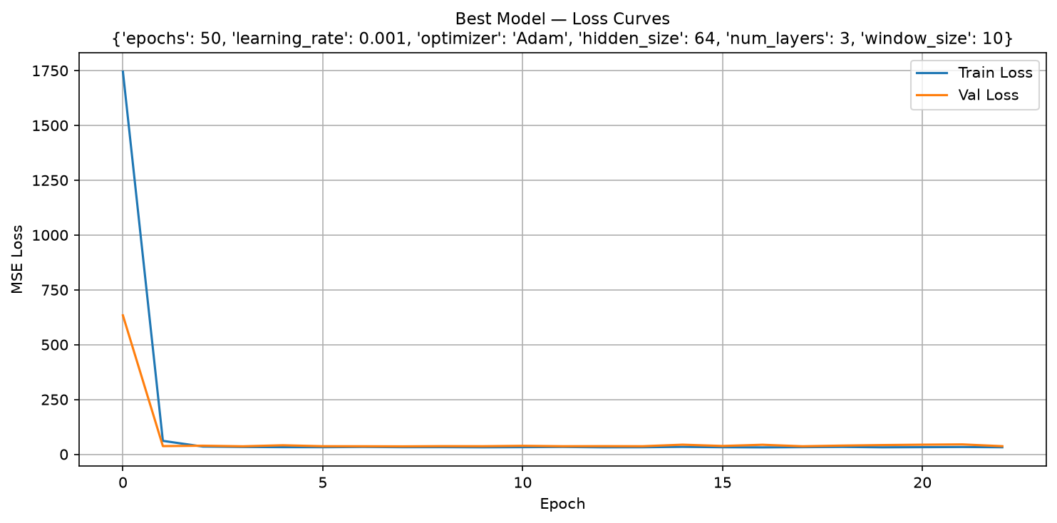
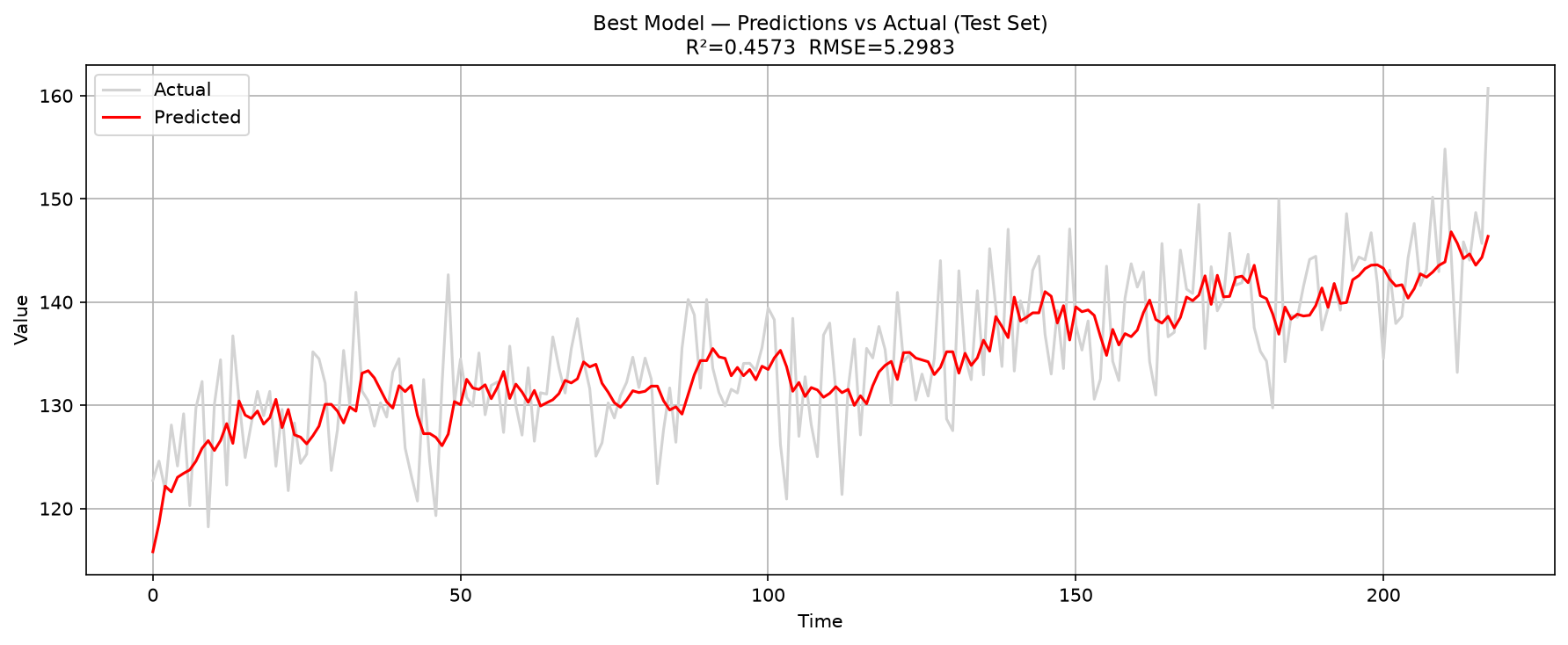
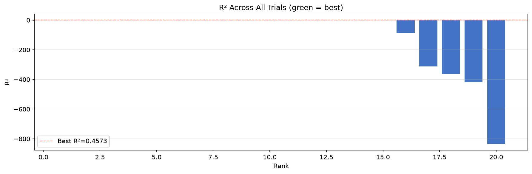
window_size column that version 10 did not have, and three charts are saved as
best_model_loss.png, best_model_predictions.png and
trial_r2_chart.png. The spreadsheet is still the useful one, because it keeps
every trial, not only the winner.
What you should see
The complete table from a real run, unedited. The Win column is the window length
for that trial.
Running 20 random trials...

Trial   Win  Epochs      LR      Opt  Hidden  Layers        R2        RMSE
------------------------------------------------------------------------------
    1    30     200   0.001     Adam      10       2    0.4358      5.3364
    2    30      50    0.01     Adam      10       2    0.4138      5.4394
    3    20      50   0.001     Adam      64       1    0.4241      5.4350
    4    50     200    0.01     Adam      10       1    0.4365      5.3207
    5    20      50     0.1      SGD      64       2  -419.3689    146.8400
    6    30      50     0.1     Adam      64       3   -86.7436     66.5462
    7    10      50     0.1     Adam      32       1    0.4351      5.4060
    8    30      50    0.01     Adam      64       3    0.4424      5.3048
    9    30     200   0.001  RMSprop      64       3    0.3956      5.5230
   10    10      50   0.001  RMSprop      64       3    0.4566      5.3021
   11    10     200   0.001      SGD      10       3  -312.0232    127.2510
   12    30     200    0.01     Adam      10       1    0.4389      5.3215
   13    20     200     0.1      SGD      32       1  -835.4003    207.1267
   14    30     100     0.1     Adam      32       2    0.4367      5.3317
   15    20      50   0.001  RMSprop      32       2    0.4163      5.4716
   16    10     100     0.1      SGD      64       2  -363.2989    137.2783
   17    10     100    0.01     Adam      10       1    0.4372      5.3959
   18    10      50   0.001     Adam      64       3    0.4573      5.2983
   19    30      50   0.001     Adam      64       2    0.4389      5.3216
   20    50      50   0.001  RMSprop      32       3    0.4393      5.3073

Best model saved → best_model.pt
Best config : {'epochs': 50, 'learning_rate': 0.001, 'optimizer': 'Adam', 'hidden_size': 64, 'num_layers': 3, 'window_size': 10}
Best R²     : 0.4573  |  MAE: 4.2199  |  RMSE: 5.2983
Results table saved → search_results.xlsx
The winner looks back only ten days. Trial 18 — 50 epochs, learning rate 0.001, Adam, 64 hidden units, 3 layers, window 10 — scored R² 0.4573 with MAE 4.2199 and RMSE 5.2983. The runner-up, trial 10, also used a window of 10 and was almost identical: 0.4566. That is our first real answer to the question the search was asked. On this data, the short look-back wins.
The gain over version 10 is small. Version 10's best was 0.4511 and version 11's is 0.4573, and part of that difference is luck of the draw rather than a better idea.
The whole program
The pieces above, put back together. This is the complete file:
import os
os.environ["KMP_DUPLICATE_LIB_OK"] = "TRUE"

import torch
import torch.nn as nn
import torch.optim as optim
from torch.utils.data import TensorDataset, DataLoader, Subset
import pandas as pd
import numpy as np
import matplotlib.pyplot as plt
import random
import itertools

# ── Reproducibility ──────────────────────────────────────────────────────────
SEED = 42
random.seed(SEED)
np.random.seed(SEED)
torch.manual_seed(SEED)

# ── Search space ─────────────────────────────────────────────────────────────
SEARCH_SPACE = {
    "epochs":       [50, 100, 200],
    "learning_rate":[0.001, 0.01, 0.1],
    "optimizer":    ["Adam", "SGD", "RMSprop"],
    "hidden_size":  [10, 32, 64],
    "num_layers":   [1, 2, 3],
    "window_size":  [10, 20, 30, 50],
}
N_TRIALS            = 20
EARLY_STOP_PATIENCE = 15
BATCH_SIZE          = 32

# ── Data ─────────────────────────────────────────────────────────────────────
df = pd.read_csv("time_series.csv")
series = df["series"].values
series_tensor = torch.tensor(series, dtype=torch.float32)

def make_loaders(window_size):
    windows      = series_tensor.unfold(0, window_size, 1)
    features     = windows[:, :-1]
    targets      = windows[:, -1:]
    full_dataset = TensorDataset(features, targets)
    total        = len(full_dataset)
    tr_end       = int(total * 0.70)
    val_end      = int(total * 0.85)
    train_loader = DataLoader(Subset(full_dataset, range(tr_end)),           batch_size=BATCH_SIZE, shuffle=True)
    val_loader   = DataLoader(Subset(full_dataset, range(tr_end, val_end)),  batch_size=BATCH_SIZE, shuffle=False)
    test_loader  = DataLoader(Subset(full_dataset, range(val_end, total)),   batch_size=BATCH_SIZE, shuffle=False)
    return train_loader, val_loader, test_loader

device = torch.device("cuda" if torch.cuda.is_available() else "cpu")

# ── Model factory ─────────────────────────────────────────────────────────────
def build_model(input_size, hidden_size, num_layers):
    layers = []
    in_dim = input_size
    for _ in range(num_layers):
        layers += [nn.Linear(in_dim, hidden_size), nn.ReLU()]
        in_dim = hidden_size
    layers.append(nn.Linear(in_dim, 1))
    return nn.Sequential(*layers).to(device)

def get_optimizer(name, params, lr):
    return {"Adam": optim.Adam, "SGD": optim.SGD, "RMSprop": optim.RMSprop}[name](params, lr=lr)

# ── Train one trial ───────────────────────────────────────────────────────────
def train_trial(cfg):
    train_loader, val_loader, test_loader = make_loaders(cfg["window_size"])
    model     = build_model(cfg["window_size"] - 1, cfg["hidden_size"], cfg["num_layers"])
    criterion = nn.MSELoss()
    optimizer = get_optimizer(cfg["optimizer"], model.parameters(), cfg["learning_rate"])

    best_val_loss = float("inf")
    best_state    = {k: v.clone() for k, v in model.state_dict().items()}
    patience_ctr  = 0
    train_losses, val_losses = [], []

    for epoch in range(cfg["epochs"]):
        # train
        model.train()
        t_loss = 0
        for xb, yb in train_loader:
            xb, yb = xb.to(device), yb.to(device)
            optimizer.zero_grad()
            loss = criterion(model(xb), yb)
            loss.backward()
            optimizer.step()
            t_loss += loss.item()
        t_loss /= len(train_loader)

        # validate
        model.eval()
        v_loss = 0
        with torch.no_grad():
            for xb, yb in val_loader:
                v_loss += criterion(model(xb.to(device)), yb.to(device)).item()
        v_loss /= len(val_loader)

        train_losses.append(t_loss)
        val_losses.append(v_loss)

        # early stopping
        if v_loss < best_val_loss:
            best_val_loss = v_loss
            best_state    = {k: v.clone() for k, v in model.state_dict().items()}
            patience_ctr  = 0
        else:
            patience_ctr += 1
            if patience_ctr >= EARLY_STOP_PATIENCE:
                break

    model.load_state_dict(best_state)
    return model, train_losses, val_losses, test_loader

# ── Evaluate on test set ──────────────────────────────────────────────────────
def evaluate(model, test_loader):
    model.eval()
    preds, actuals = [], []
    with torch.no_grad():
        for xb, yb in test_loader:
            preds.extend(model(xb.to(device)).cpu().numpy())
            actuals.extend(yb.numpy())
    p = torch.tensor(np.array(preds))
    a = torch.tensor(np.array(actuals))
    mae  = torch.mean(torch.abs(p - a)).item()
    rmse = torch.sqrt(torch.mean((p - a) ** 2)).item()
    ss_res = torch.sum((a - p) ** 2)
    ss_tot = torch.sum((a - torch.mean(a)) ** 2)
    r2 = (1 - ss_res / ss_tot).item()
    return r2, mae, rmse, preds, actuals

# ── Random search ─────────────────────────────────────────────────────────────
keys   = list(SEARCH_SPACE.keys())
combos = list(itertools.product(*SEARCH_SPACE.values()))
sampled = random.sample(combos, min(N_TRIALS, len(combos)))

results = []
best_r2    = -float("inf")
best_trial = None

print(f"Running {N_TRIALS} random trials...\n")
print(f"{'Trial':>5}  {'Win':>4}  {'Epochs':>6}  {'LR':>6}  {'Opt':>7}  {'Hidden':>6}  {'Layers':>6}  {'R2':>8}  {'RMSE':>10}")
print("-" * 78)

for i, combo in enumerate(sampled):
    cfg = dict(zip(keys, combo))
    model, t_losses, v_losses, test_loader = train_trial(cfg)
    r2, mae, rmse, preds, actuals = evaluate(model, test_loader)

    row = {**cfg, "r2": round(r2, 4), "mae": round(mae, 4), "rmse": round(rmse, 4),
           "actual_epochs": len(t_losses)}
    results.append(row)

    print(f"{i+1:>5}  {cfg['window_size']:>4}  {cfg['epochs']:>6}  {cfg['learning_rate']:>6}  "
          f"{cfg['optimizer']:>7}  {cfg['hidden_size']:>6}  {cfg['num_layers']:>6}  "
          f"{r2:>8.4f}  {rmse:>10.4f}")

    if r2 > best_r2:
        best_r2    = r2
        best_trial = {"cfg": cfg, "model": model, "t_losses": t_losses,
                      "v_losses": v_losses, "preds": preds, "actuals": actuals,
                      "r2": r2, "mae": mae, "rmse": rmse}

# ── Save best model ───────────────────────────────────────────────────────────
torch.save(best_trial["model"].state_dict(), "best_model.pt")
print(f"\nBest model saved → best_model.pt")
print(f"Best config : {best_trial['cfg']}")
print(f"Best R²     : {best_trial['r2']:.4f}  |  MAE: {best_trial['mae']:.4f}  |  RMSE: {best_trial['rmse']:.4f}")

# ── Save results table ────────────────────────────────────────────────────────
results_df = pd.DataFrame(results).sort_values("r2", ascending=False).reset_index(drop=True)
results_df.index += 1
results_df.to_excel("search_results.xlsx", index_label="Rank")
print("Results table saved → search_results.xlsx")

# ── Plots for best model only ─────────────────────────────────────────────────
# 1. Loss curves
plt.figure(figsize=(10, 5))
plt.plot(best_trial["t_losses"], label="Train Loss")
plt.plot(best_trial["v_losses"], label="Val Loss")
plt.title(f"Best Model — Loss Curves\n{best_trial['cfg']}", fontsize=11)
plt.xlabel("Epoch"); plt.ylabel("MSE Loss")
plt.legend(); plt.grid(True)
plt.tight_layout()
plt.savefig("best_model_loss.png", dpi=150)
plt.show()

# 2. Predictions vs actual
plt.figure(figsize=(12, 5))
plt.plot(best_trial["actuals"], label="Actual",    color="lightgrey", linewidth=1.5)
plt.plot(best_trial["preds"],   label="Predicted", color="red",       linewidth=1.5)
plt.title(f"Best Model — Predictions vs Actual (Test Set)\nR²={best_trial['r2']:.4f}  RMSE={best_trial['rmse']:.4f}", fontsize=11)
plt.xlabel("Time"); plt.ylabel("Value")
plt.legend(); plt.grid(True)
plt.tight_layout()
plt.savefig("best_model_predictions.png", dpi=150)
plt.show()

# 3. R² bar chart across all trials
plt.figure(figsize=(12, 4))
colors = ["#4472C4" if r < best_r2 else "#70AD47" for r in results_df["r2"]]
plt.bar(results_df.index, results_df["r2"], color=colors)
plt.axhline(best_r2, color="red", linestyle="--", linewidth=1, label=f"Best R²={best_r2:.4f}")
plt.title("R² Across All Trials (green = best)")
plt.xlabel("Rank"); plt.ylabel("R²")
plt.legend(); plt.grid(axis="y", alpha=0.4)
plt.tight_layout()
plt.savefig("trial_r2_chart.png", dpi=150)
plt.show()
Running it on your own computer
Download the zip file and unzip it
to a folder. The zip holds the programs in this series so far, the
time_series.csv data file, and pyproject.toml. This note uses
time_11.py. Open the folder in Visual Studio Code, then type these three lines
in the terminal:
uv python pin 3.12.10
uv sync
uv run time_11.py
The first line records which Python version this folder uses, and the second installs every
package that pyproject.toml lists. The third line runs the twenty trials, rebuilds
the data once per window length, and then saves the charts to disk before showing them; close
each window to continue. At the end you have best_model.pt,
search_results.xlsx and three PNG files.
Those three lines are needed only once. The next time you want to run the program again,
type just uv run time_11.py.
If you have not set up uv yet, start with How to install Visual Studio Code? and then the uv note for Windows or Mac.
What comes next
This search was still a small one: a few dozen trials, on a short list of values. Version 12 widens every range — more epochs, more learning rates, wider hidden layers, more layers — and runs 200 trials instead of 20, so the table becomes long enough to read as a landscape rather than a sample.