How to let the program search its own settings (Forecast, version 10)?
This is version 10 of the forecasting series. Version 9 compared three learning rates by hand. Version 10 lets the program do the comparison: it lists the choices for five settings, works out every combination, tries twenty of them at random, keeps the best model and saves the whole comparison as a spreadsheet. The training loop itself is unchanged; what changes is who chooses the settings.
Five settings and 243 combinations
SEARCH_SPACE = {
    "epochs":       [50, 100, 200],
    "learning_rate":[0.001, 0.01, 0.1],
    "optimizer":    ["Adam", "SGD", "RMSprop"],
    "hidden_size":  [10, 32, 64],
    "num_layers":   [1, 2, 3],
}
Each key is a setting and each list is the values worth trying. Three values in five lists give 3 × 3 × 3 × 3 × 3 = 243 possible combinations.
Trying all 243 would take hours for an improvement that would be hard to notice. Instead the
program draws N_TRIALS = 20 combinations at random from the 243. That is enough to
show which combinations perform badly, at a much lower cost.
How the search works
1. Make every combination, then draw twenty
keys   = list(SEARCH_SPACE.keys())
combos = list(itertools.product(*SEARCH_SPACE.values()))
sampled = random.sample(combos, min(N_TRIALS, len(combos)))
itertools.product builds all 243 combinations, taking one value from each list in
turn. random.sample then picks 20 of them without repeating any. The seed is fixed
at the top of the file, so the twenty chosen here are the same twenty on every run.
# ── Reproducibility ──────────────────────────────────────────────────────────
SEED = 42
random.seed(SEED)
np.random.seed(SEED)
torch.manual_seed(SEED)
2. Turn one combination into a model
def build_model(hidden_size, num_layers):
    layers = []
    in_dim = input_size
    for _ in range(num_layers):
        layers += [nn.Linear(in_dim, hidden_size), nn.ReLU()]
        in_dim = hidden_size
    layers.append(nn.Linear(in_dim, 1))
    return nn.Sequential(*layers).to(device)
Version 7's network was spelled out layer by layer. This version builds it from two numbers
instead. The loop adds one hidden layer per num_layers, each of width
hidden_size, and the last line outside the loop adds the single output:
layers.append(nn.Linear(in_dim, 1)). With
hidden_size = 64 and num_layers = 3, the result is the three-layer
network of the winning trial.
3. Train and grade each trial
for i, combo in enumerate(sampled):
    cfg = dict(zip(keys, combo))
    model, t_losses, v_losses = train_trial(cfg)
    r2, mae, rmse, preds, actuals = evaluate(model)
zip(keys, combo) pairs each setting name with its value, and dict
makes that a labelled configuration such as
{"epochs": 50, "learning_rate": 0.001, ...}. This dictionary is stored in
cfg, short for configuration: one complete set of settings for a
single trial. train_trial(cfg) then builds and trains a model using those settings.
Training works as in version 9: a trial stops early if the validation error does not improve
for 10 epochs, and the weights that gave the lowest validation error are kept. A trial that
stops improving therefore ends early instead of running to the maximum number of epochs.
4. Remember the winner and write everything out
if r2 > best_r2:
    best_r2    = r2
    best_trial = {"cfg": cfg, "model": model, ...}

torch.save(best_trial["model"].state_dict(), "best_model.pt")
results_df.to_excel("search_results.xlsx", index_label="Rank")
best_r2 starts at negative infinity, so the first trial always becomes the
benchmark and later trials must beat it to replace it. At the end two files appear: the winning
weights in best_model.pt, and every trial ranked by R² in
search_results.xlsx. The spreadsheet is the useful part, because it shows every
trial, not only the winner.
Writing the Excel file needs one extra package, openpyxl, which is why it is listed
in pyproject.toml.
What you should see
Running 20 random trials...

Trial  Epochs      LR      Opt  Hidden  Layers        R2        RMSE
----------------------------------------------------------------------
    1     200   0.001     Adam      10       2    0.4358      5.3364
    2      50    0.01     Adam      10       2    0.4138      5.4394
    3      50   0.001     Adam      64       1    0.4293      5.3670
    4     200    0.01     Adam      10       1    0.4288      5.3691
    5      50     0.1      SGD      64       2  -321.8173    127.6421
    6      50     0.1     Adam      64       3  -132.1510     81.9762
    7      50     0.1     Adam      32       1    0.4507      5.2652
    8      50    0.01     Adam      64       3    0.4467      5.2846
    9     200   0.001  RMSprop      64       3    0.4481      5.2776
   10      50   0.001  RMSprop      64       3    0.3873      5.5608
   11     200   0.001      SGD      10       3  -345.0721    132.1596
   12     200     0.1      SGD      32       1  -439.2118    149.0549
   13     100     0.1     Adam      32       2   -96.2428     70.0558
   14      50   0.001  RMSprop      32       2    0.4206      5.4075
   15     100     0.1      SGD      64       2  -389.6655    140.4165
   16     100    0.01     Adam      10       1    0.4301      5.3631
   17      50   0.001     Adam      64       3    0.4511      5.2633
   18      50   0.001     Adam      64       2    0.4489      5.2737
   19      50   0.001  RMSprop      32       3    0.4479      5.2785
   20      50     0.1     Adam      10       2    0.4333      5.3481

Best model saved → best_model.pt
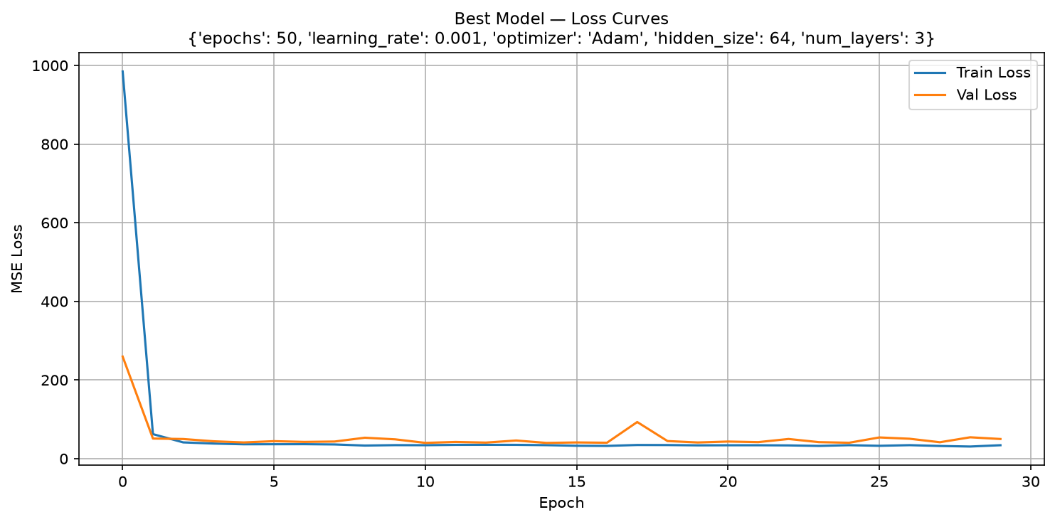
Best config : {'epochs': 50, 'learning_rate': 0.001, 'optimizer': 'Adam', 'hidden_size': 64, 'num_layers': 3}
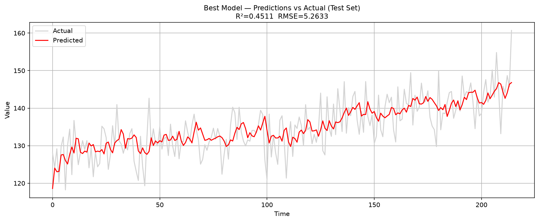
Best R²     : 0.4511  |  MAE: 4.2143  |  RMSE: 5.2633
Results table saved → search_results.xlsx
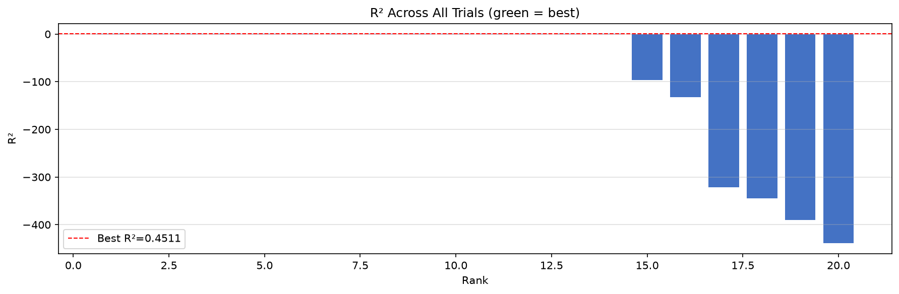
Three things in that table matter more than the winning number.
Every very poor result uses a learning rate of 0.1. Trials 5, 6, 11, 12, 13 and 15 report negative R² values in the hundreds, and RMSE in the seventies and hundreds instead of around 5. A negative R² means the model performs worse than predicting the average sales value for every day. This happens when each adjustment is too large: the weights change too much, so the errors do not become smaller. Version 9 showed a mild case of this; here it is much clearer.
The Epochs column shows the maximum allowed, not the number actually used.
Early stopping may have finished long before, and the spreadsheet keeps a column,
actual_epochs, with the real number.
The winner is only a little better than version 9. R² of 0.4511 against 0.4394. Running twenty trials produced a small improvement on top of early stopping. The honest lesson is that tuning helps a little, and no amount of tuning made this model a good one. That is a fact about the model, not about the search.
The whole program
The pieces above, put back together. This is the complete file:
import os
os.environ["KMP_DUPLICATE_LIB_OK"] = "TRUE"

import torch
import torch.nn as nn
import torch.optim as optim
from torch.utils.data import TensorDataset, DataLoader, Subset
import pandas as pd
import numpy as np
import matplotlib.pyplot as plt
import random
import itertools

# ── Reproducibility ──────────────────────────────────────────────────────────
SEED = 42
random.seed(SEED)
np.random.seed(SEED)
torch.manual_seed(SEED)

# ── Search space ─────────────────────────────────────────────────────────────
SEARCH_SPACE = {
    "epochs":       [50, 100, 200],
    "learning_rate":[0.001, 0.01, 0.1],
    "optimizer":    ["Adam", "SGD", "RMSprop"],
    "hidden_size":  [10, 32, 64],
    "num_layers":   [1, 2, 3],
}
N_TRIALS      = 20
EARLY_STOP_PATIENCE = 15   # stop if val loss doesn't improve for this many epochs
WINDOW_SIZE   = 30
BATCH_SIZE    = 32

# ── Data ─────────────────────────────────────────────────────────────────────
df = pd.read_csv("time_series.csv")
series = df["series"].values
series_tensor = torch.tensor(series, dtype=torch.float32)

def create_sliding_windows(data, window_size):
    windows  = data.unfold(0, window_size, 1)
    features = windows[:, :-1]
    targets  = windows[:, -1:]
    return features, targets

features, targets = create_sliding_windows(series_tensor, WINDOW_SIZE)
full_dataset = TensorDataset(features, targets)

total   = len(full_dataset)
tr_end  = int(total * 0.70)
val_end = int(total * 0.85)

train_loader = DataLoader(Subset(full_dataset, range(tr_end)),          batch_size=BATCH_SIZE, shuffle=True)
val_loader   = DataLoader(Subset(full_dataset, range(tr_end, val_end)), batch_size=BATCH_SIZE, shuffle=False)
test_loader  = DataLoader(Subset(full_dataset, range(val_end, total)),  batch_size=BATCH_SIZE, shuffle=False)

device = torch.device("cuda" if torch.cuda.is_available() else "cpu")

# ── Model factory ─────────────────────────────────────────────────────────────
def build_model(hidden_size, num_layers):
    input_size = WINDOW_SIZE - 1
    layers = []
    in_dim = input_size
    for _ in range(num_layers):
        layers += [nn.Linear(in_dim, hidden_size), nn.ReLU()]
        in_dim = hidden_size
    layers.append(nn.Linear(in_dim, 1))
    return nn.Sequential(*layers).to(device)

def get_optimizer(name, params, lr):
    return {"Adam": optim.Adam, "SGD": optim.SGD, "RMSprop": optim.RMSprop}[name](params, lr=lr)

# ── Train one trial ───────────────────────────────────────────────────────────
def train_trial(cfg):
    model     = build_model(cfg["hidden_size"], cfg["num_layers"])
    criterion = nn.MSELoss()
    optimizer = get_optimizer(cfg["optimizer"], model.parameters(), cfg["learning_rate"])

    best_val_loss = float("inf")
    best_state    = {k: v.clone() for k, v in model.state_dict().items()}
    patience_ctr  = 0
    train_losses, val_losses = [], []

    for epoch in range(cfg["epochs"]):
        # train
        model.train()
        t_loss = 0
        for xb, yb in train_loader:
            xb, yb = xb.to(device), yb.to(device)
            optimizer.zero_grad()
            loss = criterion(model(xb), yb)
            loss.backward()
            optimizer.step()
            t_loss += loss.item()
        t_loss /= len(train_loader)

        # validate
        model.eval()
        v_loss = 0
        with torch.no_grad():
            for xb, yb in val_loader:
                v_loss += criterion(model(xb.to(device)), yb.to(device)).item()
        v_loss /= len(val_loader)

        train_losses.append(t_loss)
        val_losses.append(v_loss)

        # early stopping
        if v_loss < best_val_loss:
            best_val_loss = v_loss
            best_state    = {k: v.clone() for k, v in model.state_dict().items()}
            patience_ctr  = 0
        else:
            patience_ctr += 1
            if patience_ctr >= EARLY_STOP_PATIENCE:
                break

    model.load_state_dict(best_state)
    return model, train_losses, val_losses

# ── Evaluate on test set ──────────────────────────────────────────────────────
def evaluate(model):
    model.eval()
    preds, actuals = [], []
    with torch.no_grad():
        for xb, yb in test_loader:
            preds.extend(model(xb.to(device)).cpu().numpy())
            actuals.extend(yb.numpy())
    p = torch.tensor(np.array(preds))
    a = torch.tensor(np.array(actuals))
    mae  = torch.mean(torch.abs(p - a)).item()
    rmse = torch.sqrt(torch.mean((p - a) ** 2)).item()
    ss_res = torch.sum((a - p) ** 2)
    ss_tot = torch.sum((a - torch.mean(a)) ** 2)
    r2 = (1 - ss_res / ss_tot).item()
    return r2, mae, rmse, preds, actuals

# ── Random search ─────────────────────────────────────────────────────────────
keys   = list(SEARCH_SPACE.keys())
combos = list(itertools.product(*SEARCH_SPACE.values()))
sampled = random.sample(combos, min(N_TRIALS, len(combos)))

results = []
best_r2    = -float("inf")
best_trial = None

print(f"Running {N_TRIALS} random trials...\n")
print(f"{'Trial':>5}  {'Epochs':>6}  {'LR':>6}  {'Opt':>7}  {'Hidden':>6}  {'Layers':>6}  {'R2':>8}  {'RMSE':>10}")
print("-" * 70)

for i, combo in enumerate(sampled):
    cfg = dict(zip(keys, combo))
    model, t_losses, v_losses = train_trial(cfg)
    r2, mae, rmse, preds, actuals = evaluate(model)

    row = {**cfg, "r2": round(r2, 4), "mae": round(mae, 4), "rmse": round(rmse, 4),
           "actual_epochs": len(t_losses)}
    results.append(row)

    print(f"{i+1:>5}  {cfg['epochs']:>6}  {cfg['learning_rate']:>6}  "
          f"{cfg['optimizer']:>7}  {cfg['hidden_size']:>6}  {cfg['num_layers']:>6}  "
          f"{r2:>8.4f}  {rmse:>10.4f}")

    if r2 > best_r2:
        best_r2    = r2
        best_trial = {"cfg": cfg, "model": model, "t_losses": t_losses,
                      "v_losses": v_losses, "preds": preds, "actuals": actuals,
                      "r2": r2, "mae": mae, "rmse": rmse}

# ── Save best model ───────────────────────────────────────────────────────────
torch.save(best_trial["model"].state_dict(), "best_model.pt")
print(f"\nBest model saved → best_model.pt")
print(f"Best config : {best_trial['cfg']}")
print(f"Best R²     : {best_trial['r2']:.4f}  |  MAE: {best_trial['mae']:.4f}  |  RMSE: {best_trial['rmse']:.4f}")

# ── Save results table ────────────────────────────────────────────────────────
results_df = pd.DataFrame(results).sort_values("r2", ascending=False).reset_index(drop=True)
results_df.index += 1
results_df.to_excel("search_results.xlsx", index_label="Rank")
print("Results table saved → search_results.xlsx")

# ── Plots for best model only ─────────────────────────────────────────────────
# 1. Loss curves
plt.figure(figsize=(10, 5))
plt.plot(best_trial["t_losses"], label="Train Loss")
plt.plot(best_trial["v_losses"], label="Val Loss")
plt.title(f"Best Model — Loss Curves\n{best_trial['cfg']}", fontsize=11)
plt.xlabel("Epoch"); plt.ylabel("MSE Loss")
plt.legend(); plt.grid(True)
plt.tight_layout()
plt.savefig("best_model_loss.png", dpi=150)
plt.show()

# 2. Predictions vs actual
plt.figure(figsize=(12, 5))
plt.plot(best_trial["actuals"], label="Actual",    color="lightgrey", linewidth=1.5)
plt.plot(best_trial["preds"],   label="Predicted", color="red",       linewidth=1.5)
plt.title(f"Best Model — Predictions vs Actual (Test Set)\nR²={best_trial['r2']:.4f}  RMSE={best_trial['rmse']:.4f}", fontsize=11)
plt.xlabel("Time"); plt.ylabel("Value")
plt.legend(); plt.grid(True)
plt.tight_layout()
plt.savefig("best_model_predictions.png", dpi=150)
plt.show()

# 3. R² bar chart across all trials
plt.figure(figsize=(12, 4))
colors = ["#4472C4" if r < best_r2 else "#70AD47" for r in results_df["r2"]]
plt.bar(results_df.index, results_df["r2"], color=colors)
plt.axhline(best_r2, color="red", linestyle="--", linewidth=1, label=f"Best R²={best_r2:.4f}")
plt.title("R² Across All Trials (green = best)")
plt.xlabel("Rank"); plt.ylabel("R²")
plt.legend(); plt.grid(axis="y", alpha=0.4)
plt.tight_layout()
plt.savefig("trial_r2_chart.png", dpi=150)
plt.show()
Running it on your own computer
Download the zip file and unzip it
to a folder. The zip holds the programs in this series so far, the
time_series.csv data file, and pyproject.toml. This note uses
time_10.py. Open the folder in Visual Studio Code, then type these three lines
in the terminal:
uv python pin 3.12.10
uv sync
uv run time_10.py
The first line records which Python version this folder uses, and the second installs every
package that pyproject.toml lists. The third line runs the twenty trials, which
takes noticeably longer than earlier versions, and then opens the charts; close each window to
continue. Two files are left behind: best_model.pt and
search_results.xlsx.
Those three lines are needed only once. The next time you want to run the program again,
type just uv run time_10.py.
If you have not set up uv yet, start with How to install Visual Studio Code? and then the uv note for Windows or Mac.
What comes next
The window length has stayed at 30 throughout, even though version 2 already showed how much it changes the shape of the examples. The next version adds it to the search space, so the program decides how far back to look as well.