How to try several learning rates and keep the best (Forecast, version 9)?
This is version 9 of the forecasting series. Until now the settings have been guesses: Adam's default learning rate, a hundred epochs, whatever weights happened to exist when the last epoch finished. Version 9 treats the learning rate as something to compare, runs the same training three times, stops each run when it stops improving, and keeps whichever model scored best.
What the learning rate does
In version 7 the optimizer adjusted every weight slightly after each batch. The learning rate controls the size of that adjustment.
- Too small — the weights change too little each time, so the model learns slowly and may still have large errors after 100 epochs.
- Too large — the weights change too much each time, so the errors may keep rising and falling instead of steadily becoming smaller.
- About right — the weights change by a suitable amount, so the model learns quickly and the errors settle at a low level.
There is no formula that tells you which value is right for a given dataset, so the practical answer is to try a few and look.
What early stopping does
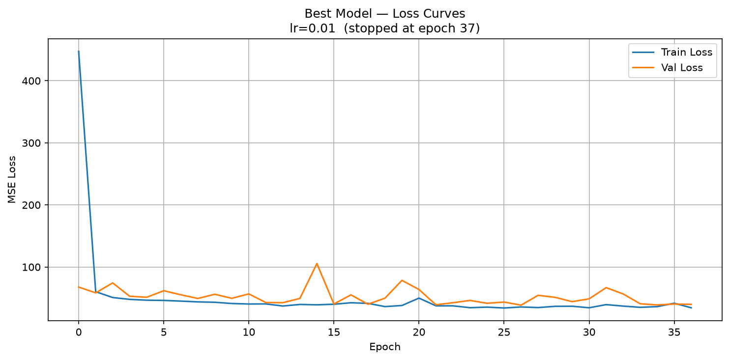
Version 8 always completed 100 epochs and used the model from the final epoch, even if the error on the validation days had started increasing earlier. One reason is that the training batches are randomly shuffled, so some weight adjustments can make predictions on the validation days worse. Version 9 checks that error after every epoch and saves the model whenever it reaches a new lowest error. If the error does not improve for 10 epochs in a row, training stops. The program then restores the saved model with the lowest validation error instead of using the model from the final epoch.
This has two benefits. Training can finish sooner when more epochs are no longer improving the model. The program also keeps the model that performed best on the validation days, not simply the model from the final epoch.
How the program works
1. Wrap one run in a function
def train_one_model(lr):
    model     = TimeSeriesModel(window_size).to(device)
    criterion = nn.MSELoss()
    optimizer = optim.Adam(model.parameters(), lr=lr)
Everything inside repeats version 7's training, with one change: lr, short for
learning rate, is now a parameter, so the same function can be called with
different learning rates. A fresh model is
built on each call, so the three runs start from independent random weights and do not
contaminate one another.
2. Keep the best weights
    best_val_loss = float('inf')
    best_state    = {k: v.clone() for k, v in model.state_dict().items()}
    patience_ctr  = 0
best_val_loss starts at infinity, so the first epoch always counts as an
improvement. best_state holds a copy of the weights at that moment. The
.clone() matters: without it the copy would keep changing as the model changed,
and there would be nothing to go back to. patience_ctr counts how many
consecutive epochs have passed without an improvement in the validation error. It starts at
zero because no epochs have run yet.
3. Stop when improvement stops
        if v_loss < best_val_loss:
            best_val_loss = v_loss
            best_state    = {k: v.clone() for k, v in model.state_dict().items()}
            patience_ctr  = 0
        else:
            patience_ctr += 1
            if patience_ctr >= PATIENCE:
                break
A new best resets the counter, patience_ctr, to zero. A worse epoch adds one to
it. When ten worse epochs have piled up in a row, break leaves the loop early. Afterwards
model.load_state_dict(best_state) puts the best weights back, so the returned model
is the one that scored best on the validation days, not the one that happened to be last.
4. Run the three learning rates
learning_rates = [0.001, 0.01, 0.1]

for lr in learning_rates:
    model, t_losses, v_losses, epochs = train_one_model(lr)
    r2, rmse, mae, preds, actuals = evaluate_on_test(model)
Each pass of the loop trains a complete model and grades it on the test days with version 8's four measures. The results are collected in a list so they can be compared and sorted afterwards.
5. Keep the winner
best = max(results, key=lambda r: r["r2"])
torch.save(best["model"].state_dict(), "best_model.pt")
max selects a result from the results list. The
key=lambda r: r["r2"] part tells Python to compare the results by their R²
values, so the result with the highest R² is stored in best.
torch.save then writes that model's learned weights to a file called
best_model.pt. A later program can load this file and reuse the model without
training it again.
What you should see
      lr   epochs        R²        RMSE         MAE
--------------------------------------------------
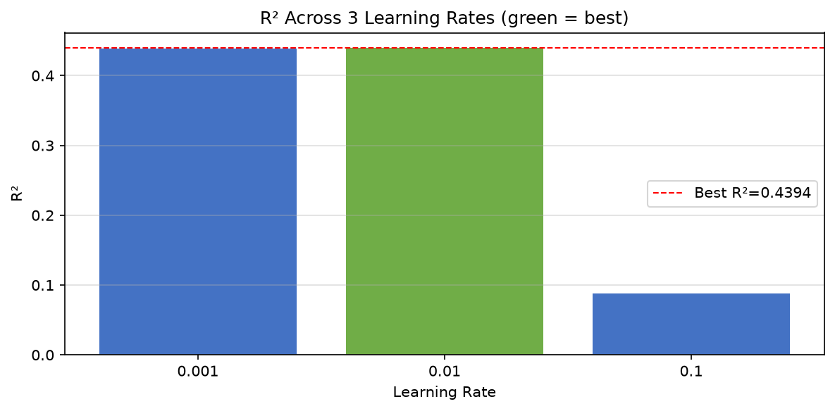
   0.001       68    0.4384      5.3538      4.2973
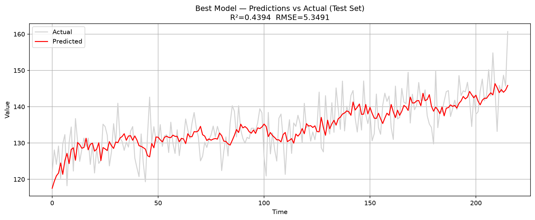
    0.01       37    0.4394      5.3491      4.2547
     0.1       12    0.0881      6.8221      5.3624

Best learning rate: 0.01  (R² = 0.4394)
Best model saved → best_model.pt
Your numbers will differ, but the pattern is what matters. The two smaller learning rates reach a similar quality, and 0.01 reaches it in 37 epochs rather than 68. Both give a similar result, but 0.01 needs fewer epochs. The large rate of 0.1 stops after 12 epochs with an R² of 0.09, because each adjustment is too large for the errors to become smaller steadily.
Two things improved since version 8. R² moved from 0.24 to about 0.44, and much of that improvement came from early stopping rather than from the learning rate: keeping the best weights instead of the final ones raises the score noticeably. Training also finishes in 37 epochs instead of 100.
The whole program
The pieces above, put back together. This is the complete file:
import os
os.environ["KMP_DUPLICATE_LIB_OK"] = "TRUE"

import torch
import torch.nn as nn
import torch.optim as optim
from torch.utils.data import TensorDataset, DataLoader, Subset
import pandas as pd
import numpy as np
import matplotlib.pyplot as plt

# ── Data preparation (same as time_08) ────────────────────────────────────────
def create_sliding_windows_with_target(data, window_size, shift=1):
    windows = data.unfold(0, window_size, shift)
    features = windows[:, :-1]
    targets = windows[:, -1:]
    return features, targets

df = pd.read_csv('time_series.csv')
series = df['series'].values
series_tensor = torch.tensor(series, dtype=torch.float32)
window_size = 30
features, targets = create_sliding_windows_with_target(series_tensor, window_size=window_size, shift=1)
full_dataset = TensorDataset(features, targets)

total_windows = len(full_dataset)
train_size = int(total_windows * 0.7)
val_size = int(total_windows * 0.15)
test_size = total_windows - train_size - val_size

train_indices = list(range(train_size))
val_indices = list(range(train_size, train_size + val_size))
test_indices = list(range(train_size + val_size, total_windows))

train_loader = DataLoader(Subset(full_dataset, train_indices),
                         batch_size=32, shuffle=True)
val_loader   = DataLoader(Subset(full_dataset, val_indices),
                         batch_size=32, shuffle=False)
test_loader  = DataLoader(Subset(full_dataset, test_indices),
                         batch_size=32, shuffle=False)

device = torch.device('cuda' if torch.cuda.is_available() else 'cpu')

# ── Visualize train/val/test split (same as time_08) ─────────────────────────
val_start = train_size
test_start = train_size + val_size
plt.figure(figsize=(12, 4))
plt.plot(range(val_start), series[:val_start], 'b-', label='Training Data')
plt.plot(range(val_start, test_start), series[val_start:test_start], 'r-', label='Validation Data')
plt.plot(range(test_start, len(series)), series[test_start:], 'g-', label='Test Data')
plt.axvline(x=val_start, color='k', linestyle='--', label='Train/Val Split')
plt.axvline(x=test_start, color='purple', linestyle='--', label='Val/Test Split')
plt.title('Time Series Train/Validation/Test Split')
plt.xlabel('Time'); plt.ylabel('Value')
plt.legend(); plt.grid(True); plt.show()

# ── Model (same as time_07/08) ────────────────────────────────────────────────
class TimeSeriesModel(nn.Module):
    def __init__(self, window_size):
        super(TimeSeriesModel, self).__init__()
        self.network = nn.Sequential(
            nn.Linear(window_size - 1, 10),
            nn.ReLU(),
            nn.Linear(10, 10),
            nn.ReLU(),
            nn.Linear(10, 1)
        )

    def forward(self, x):
        return self.network(x)

# ── NEW: training with early stopping ────────────────────────────────────────
# Early stopping: if val loss does not improve for PATIENCE consecutive epochs,
# stop training early and restore the best weights seen so far.
PATIENCE   = 10
MAX_EPOCHS = 100

def train_one_model(lr):
    model     = TimeSeriesModel(window_size).to(device)
    criterion = nn.MSELoss()
    optimizer = optim.Adam(model.parameters(), lr=lr)

    best_val_loss = float('inf')
    best_state    = {k: v.clone() for k, v in model.state_dict().items()}
    patience_ctr  = 0
    train_losses, val_losses = [], []

    for epoch in range(MAX_EPOCHS):
        # ── train ──
        model.train()
        t_loss = 0
        for batch_features, batch_targets in train_loader:
            batch_features = batch_features.to(device)
            batch_targets  = batch_targets.to(device)
            optimizer.zero_grad()
            loss = criterion(model(batch_features), batch_targets)
            loss.backward()
            optimizer.step()
            t_loss += loss.item()
        t_loss /= len(train_loader)

        # ── validate ──
        model.eval()
        v_loss = 0
        with torch.no_grad():
            for batch_features, batch_targets in val_loader:
                batch_features = batch_features.to(device)
                batch_targets  = batch_targets.to(device)
                v_loss += criterion(model(batch_features), batch_targets).item()
        v_loss /= len(val_loader)

        train_losses.append(t_loss)
        val_losses.append(v_loss)

        # ── early stopping check ──
        if v_loss < best_val_loss:
            best_val_loss = v_loss
            best_state    = {k: v.clone() for k, v in model.state_dict().items()}
            patience_ctr  = 0
        else:
            patience_ctr += 1
            if patience_ctr >= PATIENCE:
                break

    # restore the best weights
    model.load_state_dict(best_state)
    actual_epochs = len(train_losses)
    return model, train_losses, val_losses, actual_epochs

# ── NEW: evaluate on test set (returns R², RMSE, MAE) ────────────────────────
def evaluate_on_test(model):
    model.eval()
    preds, actuals = [], []
    with torch.no_grad():
        for batch_features, batch_targets in test_loader:
            preds.extend(model(batch_features.to(device)).cpu().numpy())
            actuals.extend(batch_targets.numpy())

    p = torch.tensor(np.array(preds))
    a = torch.tensor(np.array(actuals))

    mae  = torch.mean(torch.abs(p - a)).item()
    rmse = torch.sqrt(torch.mean((p - a) ** 2)).item()
    ss_res = torch.sum((a - p) ** 2)
    ss_tot = torch.sum((a - torch.mean(a)) ** 2)
    r2 = (1 - ss_res / ss_tot).item()
    return r2, rmse, mae, preds, actuals

# ── NEW: manually try 3 learning rates ────────────────────────────────────────
# Instead of picking one optimizer and one learning rate, we run the same
# training procedure three times with different learning rates and compare.
learning_rates = [0.001, 0.01, 0.1]
results = []

print(f"{'lr':>8}  {'epochs':>7}  {'R²':>8}  {'RMSE':>10}  {'MAE':>10}")
print("-" * 50)

for lr in learning_rates:
    model, t_losses, v_losses, epochs = train_one_model(lr)
    r2, rmse, mae, preds, actuals = evaluate_on_test(model)

    results.append({
        "lr": lr, "epochs": epochs,
        "r2": round(r2, 4), "rmse": round(rmse, 4), "mae": round(mae, 4),
        "model": model, "t_losses": t_losses, "v_losses": v_losses,
        "preds": preds, "actuals": actuals,
    })
    print(f"{lr:>8}  {epochs:>7}  {r2:>8.4f}  {rmse:>10.4f}  {mae:>10.4f}")

# ── Pick the best trial and save ──────────────────────────────────────────────
best = max(results, key=lambda r: r["r2"])
print(f"\nBest learning rate: {best['lr']}  (R² = {best['r2']:.4f})")

torch.save(best["model"].state_dict(), "best_model.pt")
print("Best model saved → best_model.pt")

# ── Plots ──────────────────────────────────────────────────────────────────────
# 1. Loss curves for the best trial
plt.figure(figsize=(10, 5))
plt.plot(best["t_losses"], label="Train Loss")
plt.plot(best["v_losses"], label="Val Loss")
plt.title(f"Best Model — Loss Curves\nlr={best['lr']}  (stopped at epoch {best['epochs']})")
plt.xlabel("Epoch"); plt.ylabel("MSE Loss")
plt.legend(); plt.grid(True); plt.tight_layout(); plt.show()

# 2. Predictions vs actual on test set (best trial)
plt.figure(figsize=(12, 5))
plt.plot(best["actuals"], label="Actual",    color="lightgrey", linewidth=1.5)
plt.plot(best["preds"],   label="Predicted", color="red",       linewidth=1.5)
plt.title(f"Best Model — Predictions vs Actual (Test Set)\nR²={best['r2']:.4f}  RMSE={best['rmse']:.4f}")
plt.xlabel("Time"); plt.ylabel("Value")
plt.legend(); plt.grid(True); plt.tight_layout(); plt.show()

# 3. R² bar chart comparing all 3 trials
plt.figure(figsize=(8, 4))
lrs = [str(r["lr"]) for r in results]
r2s = [r["r2"] for r in results]
colors = ["#4472C4" if r["lr"] != best["lr"] else "#70AD47" for r in results]
plt.bar(lrs, r2s, color=colors)
plt.axhline(best["r2"], color="red", linestyle="--", linewidth=1, label=f"Best R²={best['r2']:.4f}")
plt.title("R² Across 3 Learning Rates (green = best)")
plt.xlabel("Learning Rate"); plt.ylabel("R²")
plt.legend(); plt.grid(axis="y", alpha=0.4); plt.tight_layout(); plt.show()
Running it on your own computer
Download the zip file and unzip it
to a folder. The zip holds the programs in this series so far, the
time_series.csv data file, and pyproject.toml. This note uses
time_09.py. Open the folder in Visual Studio Code, then type these three lines
in the terminal:
uv python pin 3.12.10
uv sync
uv run time_09.py
The first line records which Python version this folder uses, and the second installs every
package that pyproject.toml lists. The third line trains three models in turn and
prints the comparison table, then opens the charts; close each window to continue.
Those three lines are needed only once. The next time you want to run the program again,
type just uv run time_09.py.
If you have not set up uv yet, start with How to install Visual Studio Code? and then the uv note for Windows or Mac.
What comes next
Trying three values by hand is already repetitive. The learning rate is only one setting among many — the number of hidden layers, their width, the optimizer and the window length are all choices too. The next version lets the program try many combinations by itself and keep the best.