How to train your first forecasting model (Forecast, version 7)?
This is version 7 of the forecasting series. Version 6 prepared and split the data; version 7 adds a small neural network and trains it for 100 passes through the training examples.
What the model is
The model takes the 29 recent days as input and gives back one number: its guess for the next day. Inside, it is a neural network model. We will not explain neural networks in detail in this note. A future AI Note will explain how they work.
How training works
An epoch is one complete pass through all the training examples, meaning the model has seen every example once. In each epoch the program does the same four things for every batch of 32 examples:
- Show the 29 days to the model and collect its guess.
- Compare the guess with the real next day to calculate the error, called the loss.
- Work out which weights made the loss worse and by how much.
- Adjust every weight slightly to reduce the loss.
A batch is a group of training examples processed together. In this program, a full batch contains 32 examples. The loss here is mean squared error: subtract the guess from the answer, square it, and average over the batch. Squaring makes misses count more than near misses.
After the training batches, the program measures the loss on the validation examples — the later days, which the model never learns from. Both numbers are recorded so they can be drawn.
How the program works
1. Define the network
class TimeSeriesModel(nn.Module):
    def __init__(self, window_size):
        super(TimeSeriesModel, self).__init__()
        self.network = nn.Sequential(
            nn.Linear(window_size-1, 10),  # window_size-1 because our features are window_size-1
            nn.ReLU(),
            nn.Linear(10, 10),
            nn.ReLU(),
            nn.Linear(10, 1)
        )

    def forward(self, x):
        return self.network(x)
class ... (nn.Module) is the standard way to define a PyTorch model.
__init__ builds the layers once, and nn.Sequential means run
these layers in this order. forward is what happens when the model is called:
a batch goes in, a batch of predictions comes out. With window_size = 30, the
first layer expects 29 numbers, which is exactly what the features hold.
2. Choose the loss and the optimizer
model = TimeSeriesModel(window_size)
criterion = nn.MSELoss()
optimizer = optim.Adam(model.parameters())
criterion calculates the error using mean squared error. optimizer
uses that error to adjust the model's weights. model.parameters() gives the
optimizer every weight in the network, so it knows which values it can change.
3. Pick where the work happens
num_epochs = 100
device = torch.device('cuda' if torch.cuda.is_available() else 'cpu')
model.to(device)
cuda is NVIDIA's technology for using its graphics cards to do this arithmetic
faster. On a Mac or on a laptop without an NVIDIA graphics card, the program quietly uses the
cpu instead. model.to(device)
moves the model to that place, and the batches will be moved to match.
4. The training loop
for epoch in range(num_epochs):
    model.train()
    train_loss = 0
    for batch_features, batch_targets in train_loader:
        batch_features = batch_features.to(device)
        batch_targets = batch_targets.to(device)
        outputs = model(batch_features)
        loss = criterion(outputs, batch_targets)
        optimizer.zero_grad()
        loss.backward()
        optimizer.step()
        train_loss += loss.item()
model.train() puts the network in learning mode. The inner loop walks the
training batches. For each one, model(batch_features) makes the guesses and
criterion turns them into a loss.
The next three lines help the model learn from each batch. optimizer.zero_grad()
clears the adjustment calculations from the previous batch. loss.backward()
works out how each weight should change to reduce the error. optimizer.step()
applies those changes. Repeating these three lines thousands of times is how the model learns.
5. Measure on the validation days
    model.eval()
    val_loss = 0
    with torch.no_grad():
        for batch_features, batch_targets in val_loader:
            batch_features = batch_features.to(device)
            batch_targets = batch_targets.to(device)
            outputs = model(batch_features)
            val_loss += criterion(outputs, batch_targets).item()
model.eval() switches to measuring mode, and torch.no_grad() says
do not bother working out which weights are to blame, we are not changing them here.
That saves time and memory. The validation loss is then divided by the number of batches so
that training and validation losses are on the same scale, and the pair is printed every tenth
epoch.
6. Draw two charts
plt.plot(train_losses, label='Training Loss')
plt.plot(val_losses, label='Validation Loss')
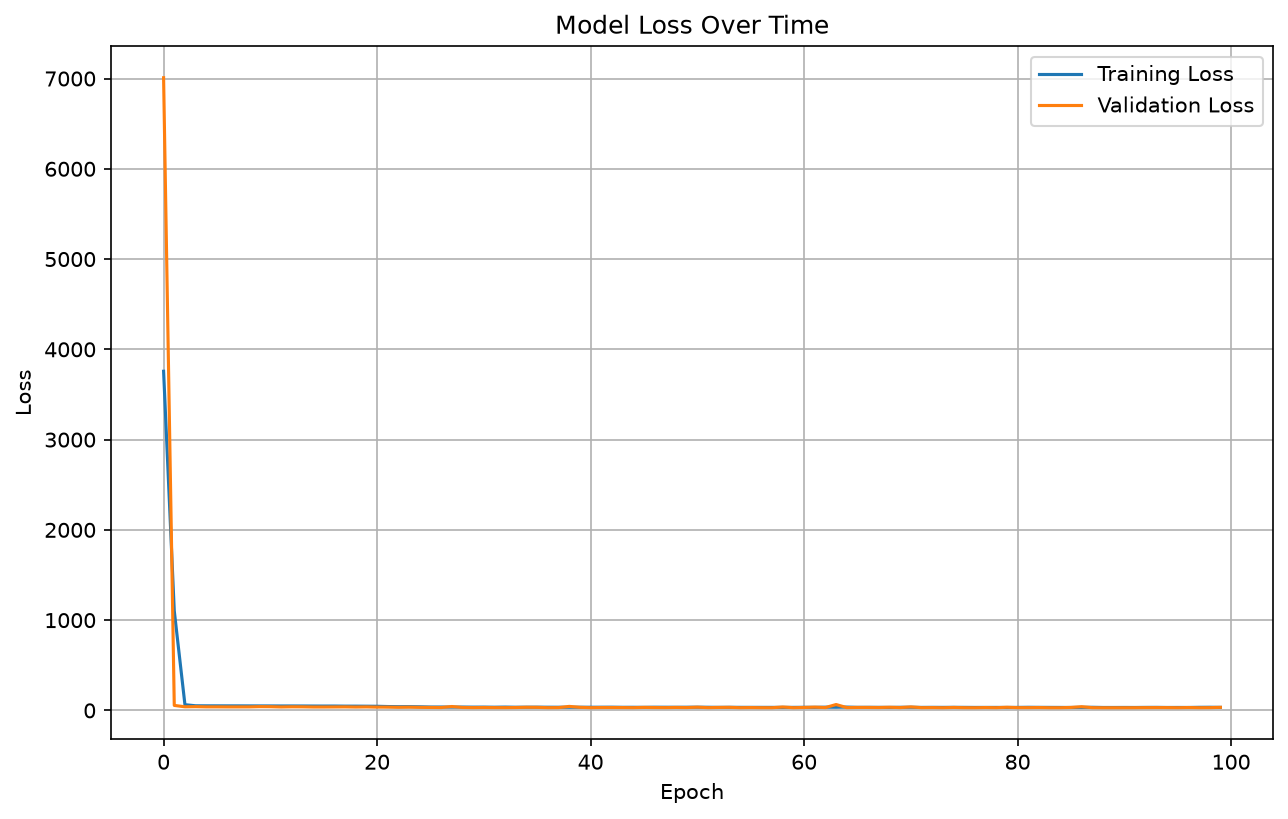
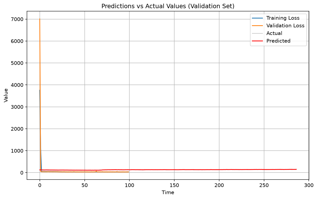
The first chart shows the two losses against epoch number: a line that should fall and then flatten. The second chart plots the model's guesses against the real validation days, grey for the truth and red for the prediction, so you can see whether the two lines sit on top of each other.
7. Reduce everything to one number
mae_torch = torch.mean(torch.abs(val_predictions_tensor - val_targets_tensor))
print(f"Validation MAE (PyTorch): {mae_torch:.4f}")
MAE, mean absolute error, is the average difference between the predictions
and the actual values, ignoring whether each prediction was too high or too low. In this run,
it is about HK$4.76. Daily sales in the validation part are around HK$140, so
(4.76 ÷ 140) × 100 ≈ 3.4%. In other words, the average
prediction error is roughly 3% of a typical day's sales. MAE is easier to explain to a manager
than the squared loss because it is measured in sales dollars.
What you should see
Epoch [10/100], Train Loss: 49.7555, Val Loss: 41.7937
Epoch [20/100], Train Loss: 46.6252, Val Loss: 38.8985
Epoch [30/100], Train Loss: 36.4138, Val Loss: 30.9879
Epoch [40/100], Train Loss: 35.3789, Val Loss: 34.1952
Epoch [50/100], Train Loss: 35.3108, Val Loss: 31.5904
Epoch [60/100], Train Loss: 33.8329, Val Loss: 30.1213
Epoch [70/100], Train Loss: 34.6491, Val Loss: 31.5292
Epoch [80/100], Train Loss: 32.7247, Val Loss: 34.9715
Epoch [90/100], Train Loss: 32.6162, Val Loss: 29.7084
Epoch [100/100], Train Loss: 33.7850, Val Loss: 34.0184
Validation MAE (PyTorch): 4.7594
Your numbers will not match these exactly. The weights start at random values, so every run takes a slightly different path downhill. What should match is the shape: both losses fall quickly at first and then wobble around a similar level.
The whole program
The pieces above, put back together. This is the complete file:
import torch
from torch.utils.data import TensorDataset, DataLoader, Subset
import pandas as pd
import matplotlib.pyplot as plt
def create_sliding_windows_with_target(data, window_size, shift=1):
    windows = data.unfold(0, window_size, shift)
    features = windows[:, :-1]  # All columns except the last
    targets = windows[:, -1:]   # Just the last column
    return features, targets

df = pd.read_csv('time_series.csv')
series = df['series'].values
series_tensor = torch.tensor(series, dtype=torch.float32)
window_size = 30
features, targets = create_sliding_windows_with_target(series_tensor, window_size=window_size, shift=1)
full_dataset = TensorDataset(features, targets)

total_windows = len(full_dataset)
train_size = int(total_windows * 0.8)  # 80% for training, 20% for validation
train_indices = list(range(train_size))
val_indices = list(range(train_size, total_windows))

train_dataset = Subset(full_dataset, train_indices)
val_dataset = Subset(full_dataset, val_indices)

# Create DataLoaders
batch_size = 32
train_loader = DataLoader(train_dataset, batch_size=batch_size, shuffle=True)
val_loader = DataLoader(val_dataset, batch_size=batch_size, shuffle=False)

import torch
import torch.nn as nn
import torch.optim as optim

# Define the model
class TimeSeriesModel(nn.Module):
    def __init__(self, window_size):
        super(TimeSeriesModel, self).__init__()
        self.network = nn.Sequential(
            nn.Linear(window_size-1, 10),  # window_size-1 because our features are window_size-1
            nn.ReLU(),
            nn.Linear(10, 10),
            nn.ReLU(),
            nn.Linear(10, 1)
        )

    def forward(self, x):
        return self.network(x)

# Initialize model, loss function, and optimizer
model = TimeSeriesModel(window_size)
criterion = nn.MSELoss()
optimizer = optim.Adam(model.parameters())

# Training loop
num_epochs = 100
device = torch.device('cuda' if torch.cuda.is_available() else 'cpu')
model.to(device)

# Lists to store losses for plotting
train_losses = []
val_losses = []

for epoch in range(num_epochs):
    # Training phase
    model.train()
    train_loss = 0
    for batch_features, batch_targets in train_loader:
        batch_features = batch_features.to(device)
        batch_targets = batch_targets.to(device)

        # Forward pass
        outputs = model(batch_features)
        loss = criterion(outputs, batch_targets)

        # Backward pass and optimize
        optimizer.zero_grad()
        loss.backward()
        optimizer.step()

        train_loss += loss.item()

    # Validation phase
    model.eval()
    val_loss = 0
    with torch.no_grad():
        for batch_features, batch_targets in val_loader:
            batch_features = batch_features.to(device)
            batch_targets = batch_targets.to(device)

            outputs = model(batch_features)
            val_loss += criterion(outputs, batch_targets).item()

    # Calculate average losses
    train_loss /= len(train_loader)
    val_loss /= len(val_loader)

    train_losses.append(train_loss)
    val_losses.append(val_loss)

    if (epoch + 1) % 10 == 0:
        print(f'Epoch [{epoch+1}/{num_epochs}], '
              f'Train Loss: {train_loss:.4f}, '
              f'Val Loss: {val_loss:.4f}')

# Plot training progress
plt.figure(figsize=(10, 6))
plt.plot(train_losses, label='Training Loss')
plt.plot(val_losses, label='Validation Loss')
plt.title('Model Loss Over Time')
plt.xlabel('Epoch')
plt.ylabel('Loss')
plt.legend()
plt.grid(True)
plt.show()

# Make predictions
model.eval()
with torch.no_grad():
    # Get predictions for validation set
    val_predictions = []
    val_targets = []
    for batch_features, batch_targets in val_loader:
        batch_features = batch_features.to(device)
        outputs = model(batch_features)
        val_predictions.extend(outputs.cpu().numpy())
        val_targets.extend(batch_targets.numpy())

# Plot predictions vs actual for validation set
plt.plot(val_targets, label='Actual', color="lightgrey")
plt.plot(val_predictions, label='Predicted', color="red")
plt.title('Predictions vs Actual Values (Validation Set)')
plt.xlabel('Time')
plt.ylabel('Value')
plt.legend()
plt.grid(True)
plt.show()

val_predictions_tensor = torch.tensor(val_predictions)
val_targets_tensor = torch.tensor(val_targets)
mae_torch = torch.mean(torch.abs(val_predictions_tensor - val_targets_tensor))
print(f"Validation MAE (PyTorch): {mae_torch:.4f}")
Running it on your own computer
Download the zip file and unzip it
to a folder. The zip holds the programs in this series so far, the
time_series.csv data file, and pyproject.toml. This note uses
time_07.py. Open the folder in Visual Studio Code, then type these three lines
in the terminal:
uv python pin 3.12.10
uv sync
uv run time_07.py
The first line records which Python version this folder uses, and the second installs every
package that pyproject.toml lists. The third line prints one line every ten
epochs, then opens the loss chart and the prediction chart; close each window for the program
to continue.
Those three lines are needed only once. The next time you want to run the program again,
type just uv run time_07.py.
If you have not set up uv yet, start with How to install Visual Studio Code? and then the uv note for Windows or Mac.
What comes next
There is a model, but its quality is judged only on the validation days, and the validation days are the last 20 per cent of the data. Version 8 adds a third, untouched part — a test set — and reports four measures on it: MAE, MSE, RMSE and R².