How to split the examples into training and validation (Forecast, version 6)?
This is version 6 of the forecasting series, and it still trains nothing. It does one thing that makes all later training trustworthy: it divides the 1,431 examples into a training part and a validation part. The model will learn from the first part and be judged on the second, which it never learns from.
Why hold examples back?
A model can score perfectly on the exact days it was trained on and still be useless, in the same way that a student who has memorised the answers to last year's paper has learned nothing about the subject. The only convincing test is a paper the student has not seen.
The validation part is that unseen paper. During training the program will keep measuring how well the model does on it, and those measurements — not the training ones — will tell you whether anything is really being learned.
Why the split is not random
The split is made in date order: the earlier examples train the model, and the latest examples validate it. The model is always judged on days that come after the days it learned from, exactly as it would be in real use.
How the program works
1. Build the same dataset as before
df = pd.read_csv('time_series.csv')
series = df['series'].values
series_tensor = torch.tensor(series, dtype=torch.float32)
print("Series tensor shape:")
print(series_tensor.shape)
window_size = 30
features, targets = create_sliding_windows_with_target(series_tensor, window_size=window_size, shift=1)
print("Features and targets shapes:")
print(features.shape)
print(targets.shape)
full_dataset = TensorDataset(features, targets)
Series tensor shape:
torch.Size([1460])
Features and targets shapes:
torch.Size([1431, 29])
torch.Size([1431, 1])2. Choose where to cut
total_windows = len(full_dataset)
train_size = int(total_windows * 0.8)  # 80% for training, 20% for validation
train_indices = list(range(train_size))
val_indices = list(range(train_size, total_windows))
len(full_dataset) is 1,431. 80% of 1,431 is 1,144.8, and
int() throws away everything after the decimal point, so train_size
becomes 1,144.
range(1144) counts 0 up to 1,143: the first 1,144 examples, the earliest days.
range(1144, 1431) counts from 1,144 to 1,430: the remaining 287 examples, the
latest days.
3. Make two views of the one dataset
train_dataset = Subset(full_dataset, train_indices)
val_dataset = Subset(full_dataset, val_indices)
Subset does not copy anything. It records a list of positions and presents the
same underlying examples through that list.
4. Make two loaders, with different shuffling
batch_size = 32
train_loader = DataLoader(train_dataset, batch_size=batch_size, shuffle=True)
val_loader = DataLoader(val_dataset, batch_size=batch_size, shuffle=False)
Each time the model goes through the training data, the training loader shuffles the order of the windows. It does not change the chronological order of the days inside each window. This helps the model learn from the sales values within the windows rather than from the order in which the windows are presented.
The validation loader keeps the examples in the same order every time. If two runs produce different error measurements for the validation days, you know that the difference is not simply because the examples were presented in a different order.
5. Print the counts
print(f"Original series length: {len(series)}")
print(f"Total number of windows: {total_windows}")
print(f"Training windows: {len(train_dataset)}")
print(f"Validation windows: {len(val_dataset)}")
Original series length: 1460
Total number of windows: 1431
Training windows: 1144
Validation windows: 2876. Draw the split
plt.plot(range(train_size), series[:train_size], 'b-', label='Training Data')
plt.plot(range(train_size, len(series)), series[train_size:], 'r-', label='Validation Data')
plt.axvline(x=train_size, color='k', linestyle='--', label='Train/Val Split Point')
plt.title('Time Series Train/Validation Split')
plt.xlabel('Time (days)')
plt.ylabel('Value')
plt.legend()
plt.grid(True)
plt.show()
The first two lines draw the sales figures in two colours: 'b-' is a blue line
for the training days, 'r-' a red line for the validation days. The third uses
plt.axvline to add a black dashed vertical line at the cut. plt.legend() prints the small key that
explains the colours, and plt.show() opens the window.
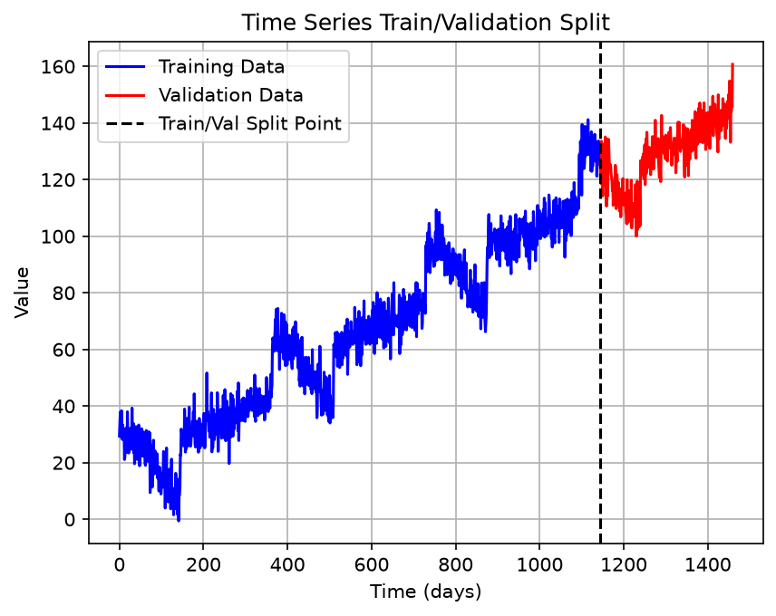
The dashed line marks the boundary: everything to its left the model may learn from, everything to its right it may only be judged on.
The whole program
The pieces above, put back together:
import torch
from torch.utils.data import TensorDataset, DataLoader, Subset
import pandas as pd
import matplotlib.pyplot as plt
def create_sliding_windows_with_target(data, window_size, shift=1):
    windows = data.unfold(0, window_size, shift)
    features = windows[:, :-1]  # All columns except the last
    targets = windows[:, -1:]   # Just the last column
    return features, targets

df = pd.read_csv('time_series.csv')
series = df['series'].values
series_tensor = torch.tensor(series, dtype=torch.float32)
print("Series tensor shape:")
print(series_tensor.shape)
window_size = 30
features, targets = create_sliding_windows_with_target(series_tensor, window_size=window_size, shift=1)
print("Features and targets shapes:")
print(features.shape)
print(targets.shape)
full_dataset = TensorDataset(features, targets)

total_windows = len(full_dataset)
train_size = int(total_windows * 0.8)  # 80% for training, 20% for validation
train_indices = list(range(train_size))
val_indices = list(range(train_size, total_windows))

train_dataset = Subset(full_dataset, train_indices)
val_dataset = Subset(full_dataset, val_indices)

# Create DataLoaders
batch_size = 32
train_loader = DataLoader(train_dataset, batch_size=batch_size, shuffle=True)
val_loader = DataLoader(val_dataset, batch_size=batch_size, shuffle=False)

print(f"Original series length: {len(series)}")
print(f"Total number of windows: {total_windows}")
print(f"Training windows: {len(train_dataset)}")
print(f"Validation windows: {len(val_dataset)}")

plt.plot(range(train_size), series[:train_size], 'b-', label='Training Data')
plt.plot(range(train_size, len(series)), series[train_size:], 'r-', label='Validation Data')
plt.axvline(x=train_size, color='k', linestyle='--', label='Train/Val Split Point')
plt.title('Time Series Train/Validation Split')
plt.xlabel('Time (days)')
plt.ylabel('Value')
plt.legend()
plt.grid(True)
plt.show()
Running it on your own computer
Download the zip file and unzip it
to a folder. The zip holds the programs in this series so far, the
time_series.csv data file, and pyproject.toml. This note uses
time_06.py. Open the folder in Visual Studio Code, then type these three lines
in the terminal:
uv python pin 3.12.10
uv sync
uv run time_06.py
The first line records which Python version this folder uses, and the second installs every
package that pyproject.toml lists. The third line prints the shapes and counts,
then opens the chart window; close it to let the program finish.
Those three lines are needed only once. The next time you want to run the program again,
type just uv run time_06.py.
If you have not set up uv yet, start with How to install Visual Studio Code? and then the uv note for Windows or Mac.
What comes next
The two parts exist and nothing has learned from either. Version 7 adds the model itself: a small network, a training loop of 100 passes, and a loss curve that shows whether the error is falling.