How to look at your sales data before forecasting (Forecast, version 1)?
This is version 1 of a series that builds, one small step at a time, a program that forecasts future sales from past sales. Version 1 contains no AI at all. It reads a file of daily sales numbers and draws one line chart. That is deliberate: before the computer can predict anything, you must first look at the data you are asking it to learn from.
Where does the data come from?
The program reads a file called time_series.csv. A CSV file is a plain text
table: each line is a row, and the values in a row are separated by commas. This file has
two columns, time and series, and 4 × 365 = 1,460 rows
— one row per day, about four years of daily sales in Hong Kong dollars.
time,series
1.0,29.395714
2.0,33.40659
3.0,37.858486
4.0,29.14184
The day numbers are written as 1.0, 2.0 and so on rather than
1, 2: the .0 marks them as decimal (floating-point)
numbers, the same kind of number as the sales figures, so the file uses one consistent
numeric format throughout.
A record of numbers arranged in time order like this is called a time series, which is where the file gets its name. Forecasting means using the first part of such a record to predict the values that come next.
How the program works
1. Load two libraries
import pandas as pd
import matplotlib.pyplot as plt
pandas is the library that reads tables, and it is given the short name
pd so the code stays compact. matplotlib is the library that draws
charts, and its plotting part is given the short name plt. Both lines are
conventions you will see in almost every data program.
2. Read the file into a table
df = pd.read_csv('time_series.csv')
series = df['series'].values
The first line reads the CSV file into df, a data frame —
pandas' name for a table with named columns. The second line picks out one column by name,
df['series'], and .values strips away the table dressing to leave
just the bare numbers: 1,460 sales figures in a row, ready to be drawn or used in calculations.
Notice what the program does not do with the time column: nothing. In
this file the rows are already in time order, so the position of a number in the list is its
time. The chart below simply plots day 1, day 2, day 3 and so on.
3. Draw the chart
plt.plot(series)
plt.title('Sales per day')
plt.xlabel('Day')
plt.ylabel('Sales-HK$')
plt.grid(True)
plt.show()
plt.plot(series) draws one line through all 1,460 numbers. The next three lines
add the finishing touches: plt.title('Sales per day') for the title,
plt.xlabel('Day') for the label under the
horizontal axis, and plt.ylabel('Sales-HK$') for the label beside the vertical
axis. plt.grid(True) adds light background lines that make it easier to
read values off the chart.
The last line, plt.show(), is what actually puts the window on your screen.
What you should see
A window opens with a line that climbs from left to right: sales start near HK$30 per day and end near HK$160, with small ups and downs along the way.
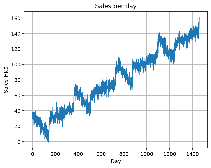
Two things are worth noticing before any forecasting begins. First, the series trends upward — later days are systematically higher than earlier ones. Second, these ups and downs are random-looking noise around that trend. Versions to come will have to deal with both facts, and seeing them with your own eyes is the reason this chart is drawn first.
The whole program
The pieces above, put back together. This is the complete file, 10 lines in all:
import pandas as pd
import matplotlib.pyplot as plt
df = pd.read_csv('time_series.csv')
series = df['series'].values
plt.plot(series)
plt.title('Sales per day')
plt.xlabel('Day')
plt.ylabel('Sales-HK$')
plt.grid(True)
plt.show()
Running it on your own computer
Download the zip file and unzip it
to a folder. The zip holds time_01.py, the time_series.csv data
file, and pyproject.toml. Open the folder in Visual Studio Code, then type
these three lines in the terminal:
uv python pin 3.12.10
uv sync
uv run time_01.py
The first line records which Python version this folder uses, and the second installs every
package that pyproject.toml lists. The third line opens the chart window; close
it to let the program finish.
Those three lines are needed only once. The next time you want to run the program again,
type just uv run time_01.py.
If you have not set up uv yet, start with How to install Visual Studio Code? and then the uv note for Windows or Mac.
What comes next
Version 1 shows the data, but a chart is not a forecast. Version 2 makes the first move towards prediction: cutting the series into sliding windows, the arrangement that turns past sales into training examples a model can learn from.